Driverless AI: Building the Perfect Predictive Model

In this Edition

• AI Series: What We've Covered?
• What is AutoML?
• What is H2O.ai?
• Walkthrough: Discovering the Best Predictive Model

AI Series: What We've Covered?

Our goal this summer was to spend more time on advanced topics, so by the time we hit the new hockey season, you have a good range of AI-related hockey analytics topics to use for your own learning and exploration.

To date, we've covered the following AI topics:

• Instant Hockey Analyses using ChatGPT and AI
• Using Linear Regression to Predict Goals
• Finding the Top Snipers using K-means Clustering
• Predicting Game Wins using Logistic Regression
• Predicting Wins using Support Vector Machine Models

In this week's newsletter, we'll introduce you to AutoML (Automated Machine Learning) and how it compares to the one-off techniques we've been applying above over the past few weeks. Further, we'll explore an open-source framework called H2O.ai – a powerful platform with model auto-discovery built into it.

What is AutoML?

AutoML is a suite of tools and techniques designed to automate the process of applying machine learning to real-world problems. AutoML makes machine learning more accessible by automating the time-consuming and complex tasks involved in developing machine learning models.

The following represent the general tasks within AutoML:

• Data Preprocessing: Automatically handling missing values, encoding categorical variables, and normalizing data.
• Feature Engineering: Generating new features or selecting the most important ones from the existing dataset.
• Model Selection: Choosing the most appropriate machine learning algorithm(s) for the task at hand.
• Hyperparameter Tuning: Optimizing the hyperparameters of the chosen model(s) to improve performance.
• Model Training and Evaluation: Training the model(s) on the dataset and evaluating their performance using various metrics.
• Ensembling: Combining multiple models to create a more robust and accurate final model.

Several benefits result from using AutoML. For example, it reduces the need for deep expertise in machine learning, making it easier for non-experts to use. Further, it saves time and computational resources by automating repetitive tasks. Also, it often yields models that are competitive with or superior to those manually crafted by experts. And lastly, it provides a systematic approach to model development, reducing the risk of human error.

If you compare AutoML with what we've been writing about over the past few weeks, AutoML reduces the need to conduct individual tests to discover which algorithm creates the best model. For example, over the last two weeks we tested Logistic Regression and Support Vector Machine (SVM) and the predictive accuracy and strength of those models was 70% and 79% respectively. However, you can use AutoML to discover the top-performing models without the need to run parallel, exploratory model-building exercises.

What is H2O.AI?

H2O.ai is an open-source machine learning and AI platform that provides tools for building and deploying predictive models and machine learning applications. H2O.ai provides several components that automate many aspects of the model-building process. H2O.ai offers a variety of products, including H2O-3, Driverless AI, and H2O Q.

H2O.ai's AutoML includes:

• Support for supervised learning tasks (classification and regression).
• Automatic data splitting and cross-validation.
• Stacked ensembles for improved performance.
• Comprehensive leaderboard to compare models.

There are three key components to H2O.ai, which are listed below.

1. H2O-3: An open-source distributed machine learning platform that provides scalable and fast implementations of common machine learning algorithms.
2. Driverless AI: An automated machine learning (AutoML) platform that automates various aspects of the data science workflow, from data preprocessing and feature engineering to model tuning and deployment.
3. H2O Q: An AI App development framework for creating data science applications without requiring extensive programming skills.

AutoML, generally, and specifically H2O.ai are versatile in the ways you can apply them. Below are some general use cases where you can use H2O.ai.

• Predictive Analytics: Building models to predict outcomes based on historical data.
• Natural Language Processing (NLP): Analyzing and processing text data for applications such as sentiment analysis and text classification.
• Time Series Forecasting: Predicting future values based on past data trends.
• Anomaly Detection: Identifying unusual patterns or outliers in the data.
• Customer Segmentation: Grouping customers based on behavior and characteristics for targeted marketing.

Within these use cases, there is a standard workflow that H2O.ai manages to optimize the modeling process. A lot of this is automated, which is why it's called Driverless AI. Below is an overview of the steps within the H2O.ai platform:

Data Preprocessing: H2O Driverless AI automatically handles data cleaning, missing value imputation, and normalization. It can perform advanced data augmentation and feature generation.

Feature Engineering: Driverless AI generates and selects the most relevant features automatically. It uses techniques like target encoding, frequency encoding, and interaction features to enhance the model’s predictive power.

Model Selection: H2O.ai evaluates multiple algorithms and selects the best-performing ones based on the problem at hand. Algorithms include gradient boosting, random forests, generalized linear models, and deep learning.

Hyperparameter Optimization: H2O.ai optimizes hyperparameters using techniques such as grid search and random search, along with proprietary optimization methods. This ensures the model is fine-tuned for the best performance.

Model Evaluation: H2O.ai provides detailed model performance metrics, such as accuracy, precision, recall, F1-score, and AUC-ROC. It also offers explainability features, allowing users to understand the contribution of each feature to the model’s predictions.

Deployment: Models built with H2O.ai can be easily deployed as APIs for real-time predictions. The platform supports integration with various cloud environments and on-premise infrastructures.

In the next section, we'll demonstrate how you can use H2O.ai to find the best-performing classification model. The goal will be to beat 79% (the SVM model).

Walkthrough: Discovering the Best Predictive Model

There are two resource files that accompany this walkthrough:

• AutoML Hockey Stats (Game-Level) Dataset
• H2O R Code

Download these files into a newly created folder on your local machine.

When the files are downloaded, create a new R Project in RStudio. To do this:

• Open RStudio.
• Click File, New Project.
• Select Existing Project, navigate to the folder you created above, and click Create Project.
• After the new project is created, click File, New File, R Markdown.
• Provide a title for the new file and click OK.

The first step is to add the R libraries you'll need for this walkthrough. The code snippet below shows each of these libraries.

library(h2o)
library(ggplot2)
library(dplyr)
library(reshape2)
library(kableExtra)
library(broom)

The first step when using H2O.ai is to initiate a session by using the h2o.init() function. You then load the CSV file you downloaded and print out the head of the file to confirm that it loaded correctly.

h2o.init()

data_file <- "automl_classification_game_data.csv"

game_stats_data <- h2o.importFile(data_file)

print(head(game_stats_data))

In the next step, you'll identify the response variable (WIN) and predictor variables. Using the setdiff() function, you can also filter out the DATE, TEAM and response (i.e., WIN) variables.

response <- "WIN"

predictors <- setdiff(names(game_stats_data), c("DATE", "TEAM", response))

print(predictors)

This next code snippet recasts the response variable as a factor and then creates a training and test data set.

game_stats_data[[response]] <- as.factor(game_stats_data[[response]])

print(h2o.levels(game_stats_data[[response]]))

splits <- h2o.splitFrame(game_stats_data, ratios = 0.8, seed = 1234)
train <- splits[[1]]
test <- splits[[2]]

The next code snippet configures the AutoML process by using the h2o.automl() function. The parameters for this function are the WIN column (response), the predictor columns (predictors), the training dataset, number of models and seed. Note that the more models you add here, the longer H2O.ai will take to process the AutoML request. The result of the AutoML process is the leaderboard (lb), which you can recast as a data frame and print out.

aml <- h2o.automl(y = response,
                  x = predictors,
                  training_frame = train,
                  max_models = 20,
                  seed = 1234)

lb <- aml@leaderboard

lb_df <- as.data.frame(lb)

print(lb_df)

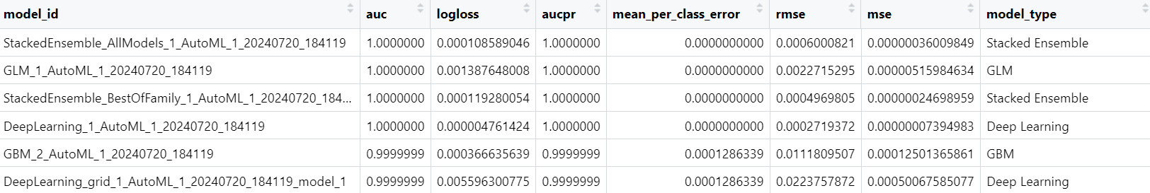
Below is a snapshot of the first few models produced by the H2O.ai platform along with key performance metrics – which are showing some very strong performance numbers.

The next code snippet cleans up the data frame and saves it as a CSV file, so we can use it offline. For example, you can use the CSV leaderboard file to create a report to share with your colleagues or management.

lb_df$model_type <- sapply(lb_df$model_id, function(x) {
  if (grepl("StackedEnsemble", x)) {
    return("Stacked Ensemble")
  } else if (grepl("GLM", x)) {
    return("GLM")
  } else if (grepl("GBM", x)) {
    return("GBM")
  } else if (grepl("DeepLearning", x)) {
    return("Deep Learning")
  } else if (grepl("DRF", x)) {
    return("Distributed Random Forest")
  } else if (grepl("XRT", x)) {
    return("Extremely Randomized Trees")
  } else {
    return("Other")
  }
})

print(lb_df)

colnames(lb_df) <- c("MODEL_ID", "AUC", "LOG_LOSS", "AUC_PR", 
                                           "MEAN_PCE", "RMSE", "MSE", "MODEL_TYPE")

lb_df$LOG_LOSS <- round(lb_df$LOG_LOSS, 6)
lb_df$MEAN_PCE <- round(lb_df$MEAN_PCE, 6)
lb_df$RMSE <- round(lb_df$RMSE, 6)
lb_df$MSE <- round(lb_df$MSE, 6)

write.csv(lb_df, "automl_leaderboard_summary.csv", row.names = FALSE)

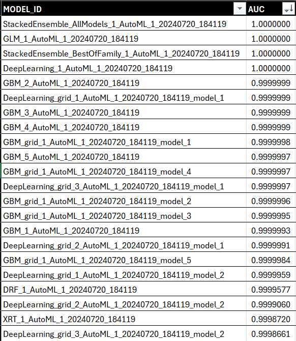
When you open the CSV in Excel and sort on the AUC column, you see a ranked view of the best-performing models that H2O.ai produced using your dataset and hyperparameters. The top model is a Stacked Ensemble model, which is an advanced ensemble learning technique that combines multiple machine learning models to improve predictive performance.

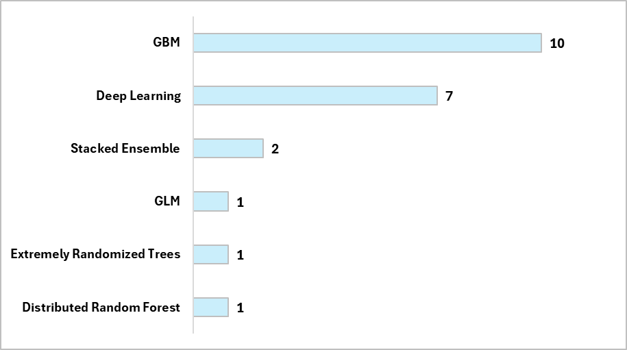
To get a sense for the type of models in the leaderboard, we created a quick PivotTable and chart, which you can see below.

With ten in the leaderboard, the GBM (Gradient Boosting Machine) model is a powerful machine learning technique used for regression and classification tasks. It builds an ensemble of decision trees in a sequential manner, where each new tree is constructed to correct the errors made by the previous trees.

With seven on the leaderboard, the Deep Learning models are based on neural networks, specifically deep neural networks with multiple layers (hence the term "deep"). Deep Learning models are neural network-based models that excel in tasks involving complex, high-dimensional data but require large datasets and significant computational resources.

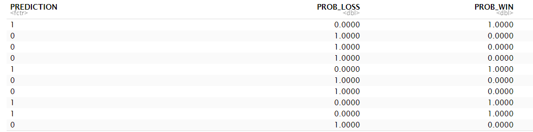
The next code snippet takes the best model (aml@leader) uses it to predict the results using the test dataset. We then create a data frame for the predictions (predictions_df), clean up the data formatting and print the results to the console to validate the results.

best_model <- aml@leader

pred <- h2o.predict(best_model, test)

predictions_df <- as.data.frame(pred)

colnames(predictions_df) <- c("PREDICTION", "PROB_LOSS", "PROB_WIN")

options(scipen = 999)

predictions_df$PROB_LOSS <- round(predictions_df$PROB_LOSS, 6)
predictions_df$PROB_WIN <- round(predictions_df$PROB_WIN, 6)

print(predictions_df)

The below are the first ten rows of the predictions data frame.

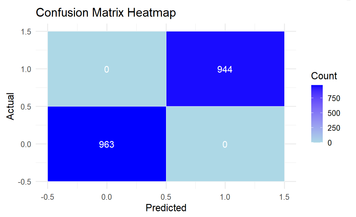
It's tough to make sense of the predictions data frame, so we created a confusion matrix. Note that you can use the basic confusion matrix in H2O.ai (using the h2o.confusionMatrix() function), or you can create a cleaner, more aesthetic version of the confusion matrix – which is what we did below.

perf <- h2o.performance(best_model, newdata = test)
confusion_matrix <- h2o.confusionMatrix(perf)

confusion_matrix_df <- as.data.frame(confusion_matrix)
sub_confusion_matrix_df <- confusion_matrix_df[0:2]

sub_confusion_matrix_df_2 <- confusion_matrix_df[1:2, 1:2]

print(sub_confusion_matrix_df_2)

melted_confusion_matrix <- melt(as.matrix(sub_confusion_matrix_df_2))

heatmap_plot <- ggplot(data = melted_confusion_matrix, aes(x = Var2, y = Var1, fill = value)) +
  geom_tile(color = "white") +
  scale_fill_gradient(low = "lightblue", high = "blue") +
  geom_text(aes(label = value), color = "white", size = 5) +
  labs(title = "Confusion Matrix Heatmap",
       x = "Predicted",
       y = "Actual",
       fill = "Count") +
  theme_minimal(base_size = 15)

print(heatmap_plot)

The result is a confusion matrix showing a perfect model – which if you remember is the best-performing model from the H2O.ai leaderboard.

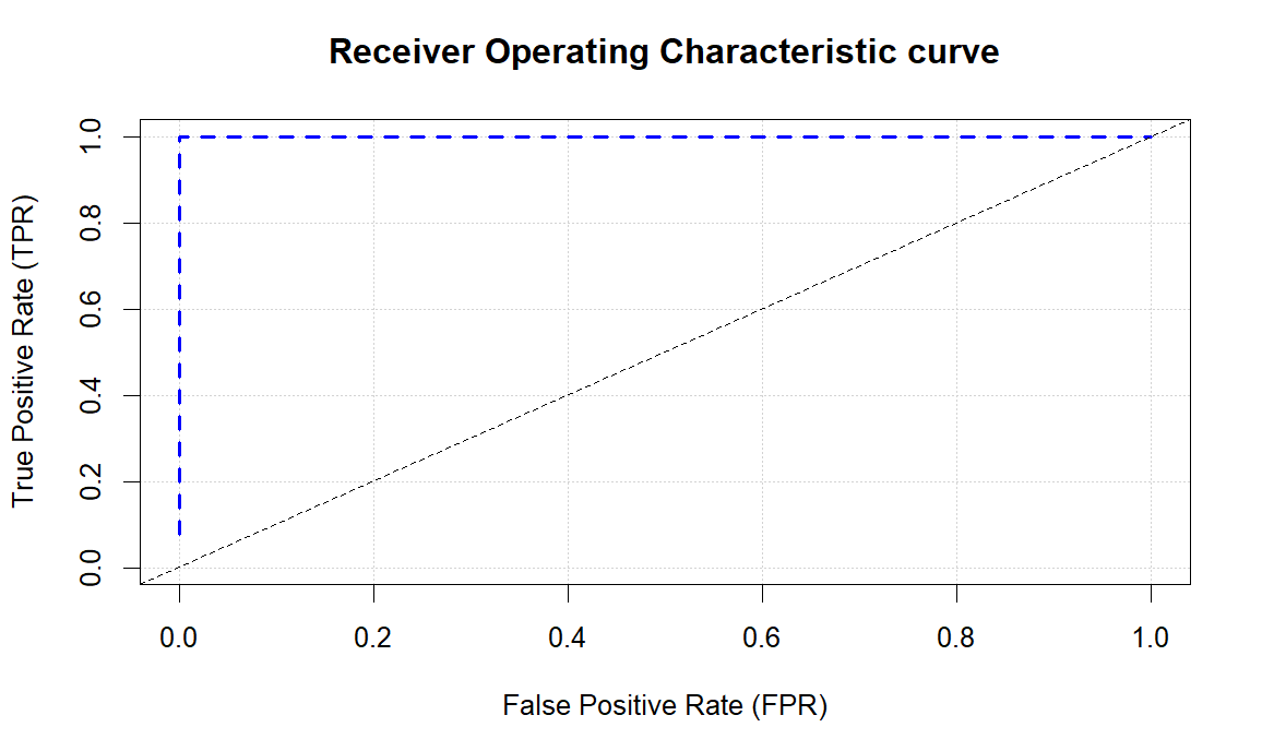
The final step is to plot the ROC curve, which is what the code snippet does below.

plot(perf, type = "roc")

The result of this shows the strength of the ROC curve with a very strong AUC.

Check out our quick-hit YouTube video below.

So, to summarize:

• We used H2O.ai to implement AutoML to test and deliver a top-performing predictive model (Win/Lose).
• H2O.ai returned a leaderboard, where the top-performing model was a near-perfect model.
• This means that this model could potentially predict a win or loss when applied to similar datasets in the real world.

However, as with any machine learning project, don't pop the champagne too early! Creating a near-perfect model with H2O.ai or any other machine learning platform can be both a positive and a negative sign. With a near-perfect model, we would recommend some additional steps you should take to ensure the validity and reliability of the model.

Below are some of the reasons why you might end up with a perfect predictive model.

• Overfitting: The model might have overfit the training data, capturing noise and specific patterns that do not generalize to new, unseen data.
• Data Leakage: Your dataset might have information that unintentionally gives away the target variable, leading to artificially high performance.
• Insufficient Complexity: If your data is too simple or has clear separations between classes, even basic models can achieve near-perfect accuracy.
• High-Quality Data: It is possible that your data is exceptionally clean, well-labeled, and relevant, resulting in a high-performing model.
• Cross-Validation Issues: If the cross-validation or validation strategy is not properly implemented, it can give misleadingly high performance metrics.

In our next newsletter, we'll cover off on some of the practical ways in which you can test/re-test your model and confirm if you truly do have a perfect model or there are other issues at play.

Summary

In this week's newsletter, we introduced you to the concept of AutoML, which is a more efficient way of building and testing machine learning models. We also introduced you to a specific AutoML platform/framework called H2O.ai. H2O.ai is an open-source and is often characterized as Driverless AI because of the way in which it automates key AI tasks.

We then used the H2O.ai framework to create a set of predictive models using the same game stats dataset we've been using over the last couple of weeks – i.e., for the Logistic Regression model and the SVM model. If you recall, the Logistic Regression produced a 70% model and SVM produced a 79% model. The dataset and code can be found at the links below:

• AutoML Hockey Stats (Game-Level) Dataset
• H2O R Code

Comparatively, H2O.ai produced a perfect model at 100%. There could be various reasons for this, so in our next newsletter we'll explore why machine learning can produce perfect models and what to do if you find yourself in this situation.

Subscribe to our newsletter to get the latest and greatest content on all things hockey analytics!