Preparing for the NHL Draft 2024: Team Analysis

In this Edition

• Newsletter Series Recap
• Getting the Data
• Exploring Trends using PivotTables
• Analyzing the Offense, Defense and Goaltending Scores
• What Teams Need the Most Help?

Newsletter Series Recap

This is the third week in our six-week newsletter series on Preparing for the NHL Draft 2024. In the first two editions, we covered the following topics:

• Week 1 Edition: Introduction to the six-week series and getting you started with the first dataset.
• Week 2 Edition: Overview of the process of data discovery using Microsoft Excel and a high-level walkthrough using the team stats dataset.

In this week's edition, we'll continue the analysis of the NHL teams using the multi-season data and focus on three areas: Offense, Defense and Goaltending. To do this, we've created three composite metrics using a subset of the team stats.

You can think of these composite metrics as directional and not comprehensive. We've also normalized the scores so they fall between 0 and 1 and we've created quartiles. Lower-performing teams fall into quartiles 1 and 2, and higher-performing teams fall into quartiles 3 and 4.

Using the three categories, we'll do three things:

1. Explore trends using PivotTables;
2. Analyze the team-level scores; and
3. Group and cluster teams to classify strongest to weakest.

So, let's get started!

Getting the Data

In the original dataset, we collected six seasons worth of data. We collected the raw data from Hockey-Reference and then added some of our own calculated metrics. After exploring the data, we noticed statistical anomalies in 2019-2020 and 2020-2021 – primarily attributed to COVID. For example, below you can see the average goals across the six seasons with the dip across these two seasons.

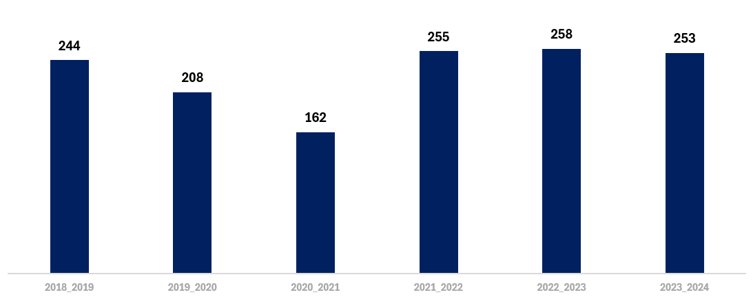
Therefore, we filtered for the 2021-2022, 2022-2023 and 2023-2024 seasons as our starting point for this week's dataset, which you can find here. This includes the summary stats data for three seasons along with the offense, defense and goaltending composite metrics and associated quartiles.

Exploring Trends using PivotTables

PivotTables are useful for exploring data to discover trends, patterns and potentially interesting metrics. For this week's analysis, we used PivotTables to explore high-level and team-specific trends.

High-Level Trend Analysis

In the high-level analysis, you can see the league average for each of offense, defense and goaltending across the three seasons. The visualization shows:

• Offense was generally consistent, though was a bit higher in the 2022-2023 season.
• Defense was generally consistent, though was a bit lower in the 2022-2023 season.
• Goaltending was higher in the 2021-2022 season, but dropped to consistent levels across 2022-2023 and 2023-2024.

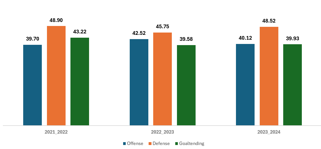
While this is vaguely interesting from a high-level trend perspective, it doesn't reveal much about each of the teams. And because we want to get at which teams are strong and which ones are weak, we need to step one level down.

Team-Level Analysis

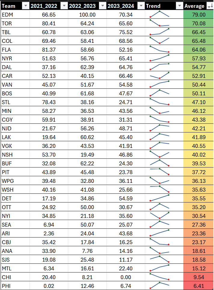
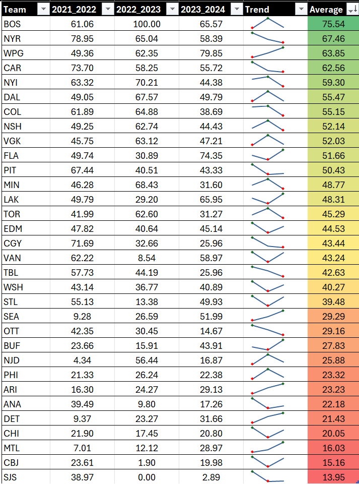
In the next three views (offense, defense and goaltending respectively), we've created a team-level analysis. We first used the PivotTable functionality to pivot TEAM_ABBR as the rows, SEASON as the columns and OFFENSIVE, DEFENSIVE and GOALTENDING as the Values (using Average rather than Sum). We created one PivotTable for each of these and then added a Trend column (using the Sparkline feature in Excel).

Offense

The first view below is for the Offense metric. In this view, we can see that Edmonton are outperforming the league by 9 points (likely because of their stand-out results in 2022-2023), there's a high-performing cohort in the league (teams greater than 64%), and there's a significant delta between Edmonton's average and Philadelphia's average. The Trend column shows the trending across each of the seasons for each team, and you can also see that only ten teams are above 50%.

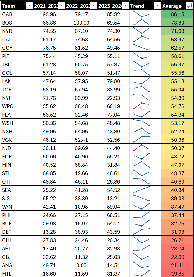
Defense

This next view is for the Defense metric, and here again we see the usual suspects with a couple of exceptions – for example, Pittsburgh and Calgary. Interestingly, the drop from Carolina's stellar average to below 60 points happens quickly – with most of the league falling below 60%. And again, we see a significant delta between Carolina at the top and Montreal at the bottom.

Goaltending

And lastly, this next view is for our Goaltending metric. For those in the statistical basement, we're beginning to see a trend. But, we're also seeing that some of the better teams in Offense and Defense are not as strong here – for example, Edmonton and Florida.

The above views are useful in that they give you some trending over three seasons worth of data across Offense, Defense and Goaltending. You would of course need to dig into the individual team data and look at other factors, such as age, depth of talent, injuries, coaching, and so on to really understand why teams are performing the way they are.

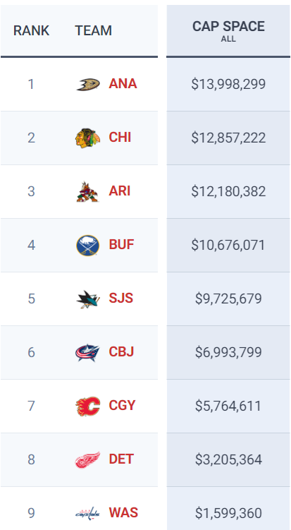
Note: We were curious on cap, so we looked at the salary cap space for those teams that were low performers. We discovered many of them had come in under the cap space. For example, see below for the top ten teams in 2023-2024 that came in under the cap space and compare them with the lower-performing teams.

Let's now look at the numbers associated with each team, with the end goal of identifying those teams that are most in need of help.

Analyzing the Offense, Defense & Goaltending Scores

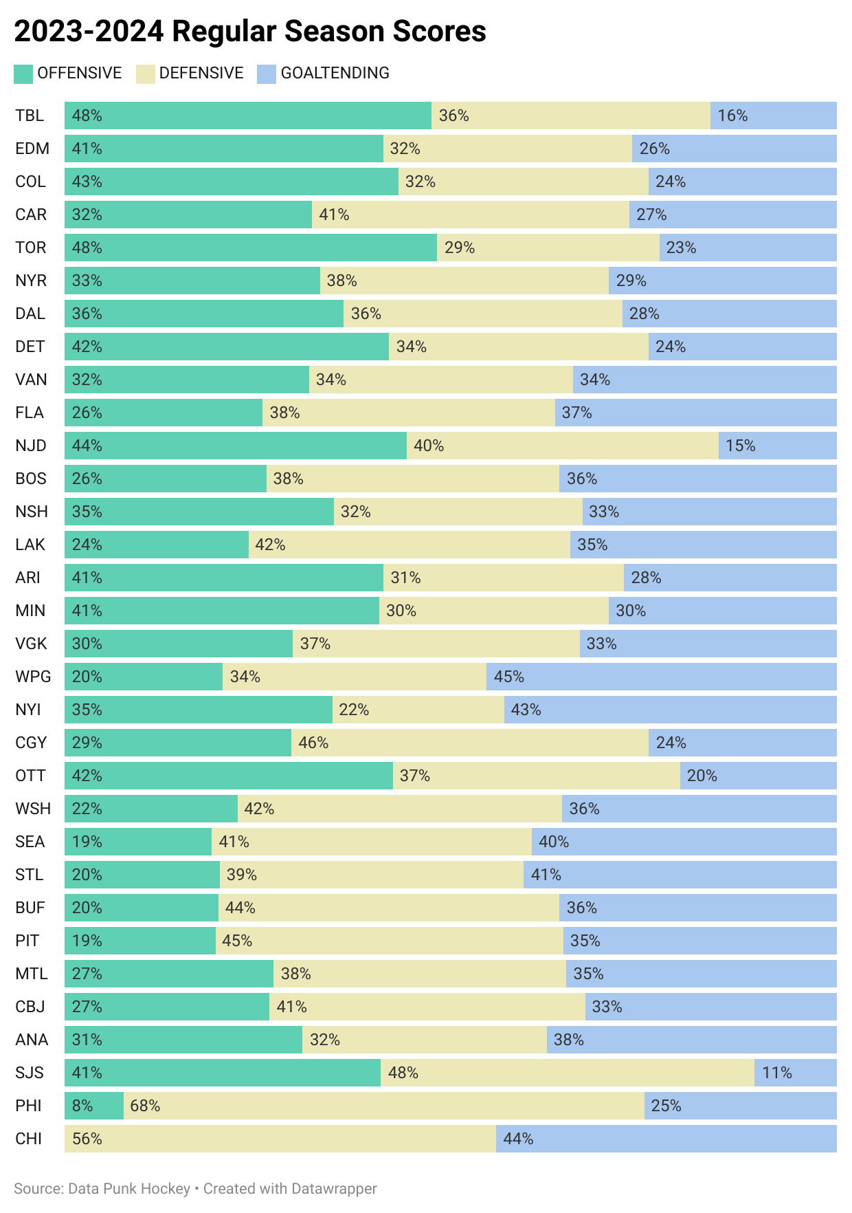
To start our analysis, we filtered for the 2023-2024 season and created a horizontal 100% stacked column chart.

What's interesting here is that there is no evenly split team – meaning the three categories split across 33.3% offense, 33.3% defense and 33.3% goaltending. Each team has a different balance across these three metrics. However, your eyes should be drawn to the teams that have dramatically lower proportions. For example, Chicago has 0% offense, Philadelphia has 8% offense, and San Jose has 11% goaltending. We would read these as outliers that flag a team for potential issues that need to be addressed.

While this is an interesting summary view, we need to more deeply explore each of the composite scores.

Offense Scores

In this next visualization, you can see the team abbreviation (TEAM_ABBR), the offense score (OFFENSIVE) and the quartile OFFENSIVE_Q). If you sort the OFFENSIVE column in ascending order, you'll see how the lower-performing teams ranked higher along with their corresponding quartile. We've called out the OFFENSIVE scores in quartiles 1 and 2 in red; we believe that these teams would need some offensive help when looking at the incoming draft prospects.

You could draw your own line here – say, only use quartile 1; however, in quartile 2 there are some similar lower-performing teams. For example, Montreal, Buffalo, St. Louis, Seattle and Washington are all within 3.5% of one another.

Another way to analyze this data is to use a K-Means cluster, a machine-learning algorithm that uses Euclidean distance to create clusters. Here, you can see cluster #3 includes thirteen low-performing teams.

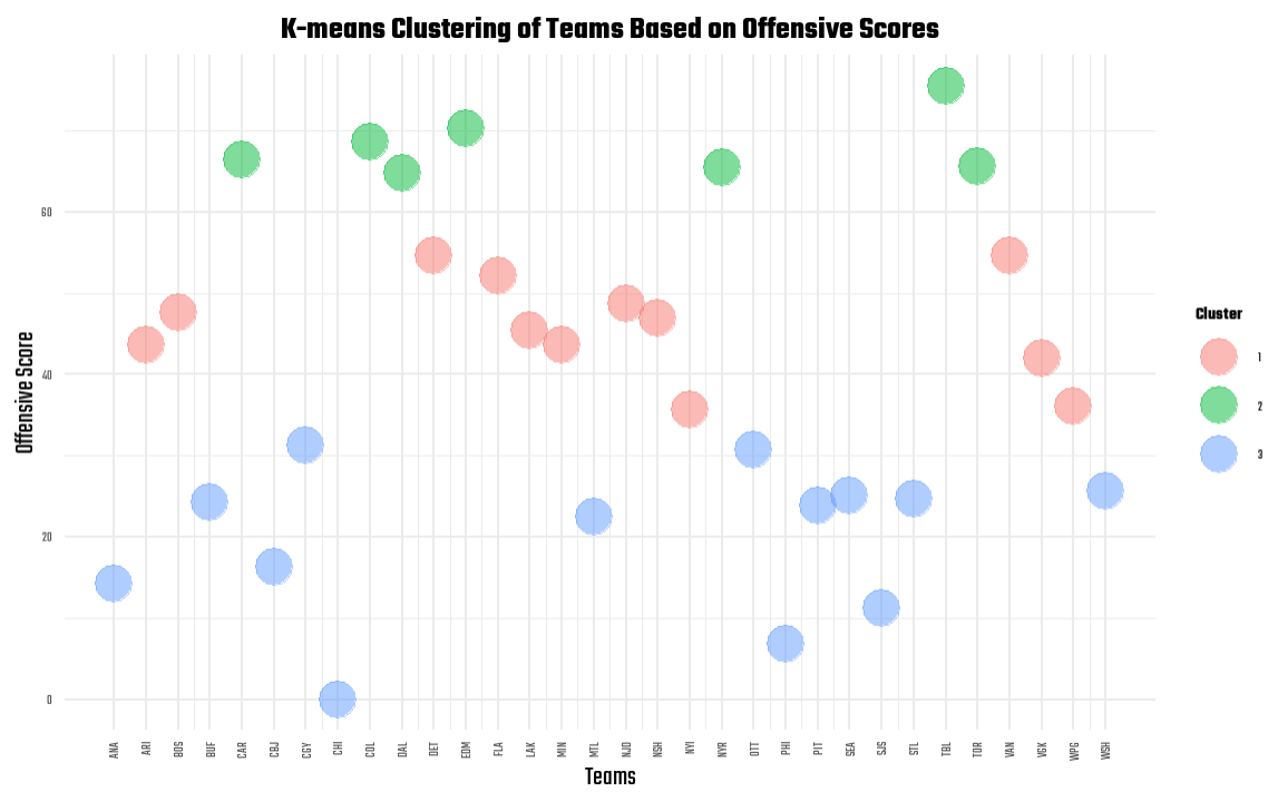
If we favor the clustering algorithm, the teams most needing offensive help are 1) Anaheim, 2) Buffalo, 3) Columbus, 4) Calgary, 5) Chicago, 6) Montreal, 7) Ottawa, 8) Philadelphia, 9) Pittsburgh, 10) Seattle, 11) San Jose, 12) St. Louis, and 13) Washington

Defense Scores

We created a similar view for the defense scores. Here again, you can sort on the DEFENSIVE column and explore those teams that are lower-performing defensively along with their respective quartiles. It's more difficult to draw the line using the quartiles here because there is a tighter statistical grouping in the mid-forties.

However, if we run the data through the K-Means clustering algorithm, the resulting cluster shows nine teams that may need defensive help.

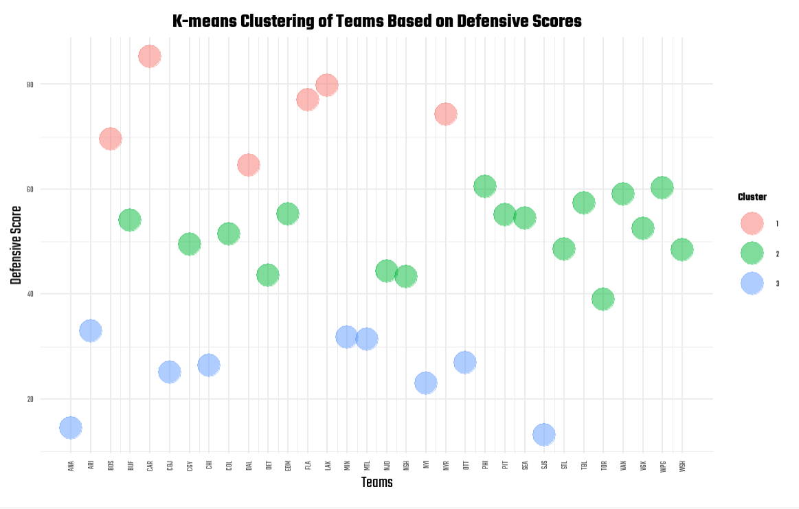
These teams are 1) Anaheim, 2) Arizona, 3) Columbus, 4) Chicago, 5) Minnesota, 6) Montreal, 7) New York Islanders, 8) Ottawa, and 9) San Jose.

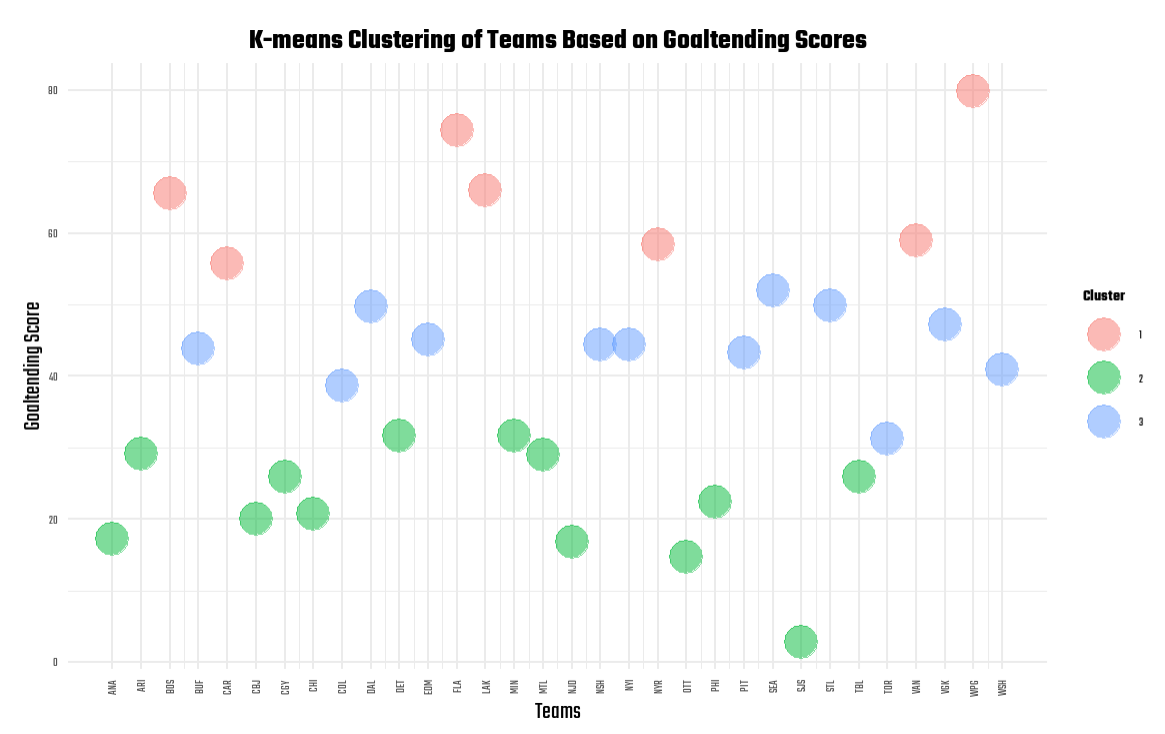
Goaltending Scores

Lastly, let's look at goaltending. Again, we created a view where you can sort on GOALTENDING and view the associated quartile. Small jumps in the statistics are evident here – especially within the second quartile, which would lead us to potentially take all teams from quartile 1 but not all teams from quartile 2.

But, let's once again verify using the K-Means clustering algorithm. The resulting teams are 1) Anaheim, 2) Arizona, 3) Columbus, 4) Calgary, 5) Chicago, 6) Detroit, 7) Minnesota, 8) Montreal, 9) New Jersey, 10) Ottawa, 11) Philadelphia, 12) San Jose, and 13) Tampa Bay.

What Teams Need the Most Help?

Based on our analysis above, the following table provides a view of those teams that need the most help across offense, defense and goaltending.

In this table, you can see that the first six teams are those with the highest need (they performed low across offense, defense and goaltending). The next four are weaker in two areas. And the final nine are weaker in one area.

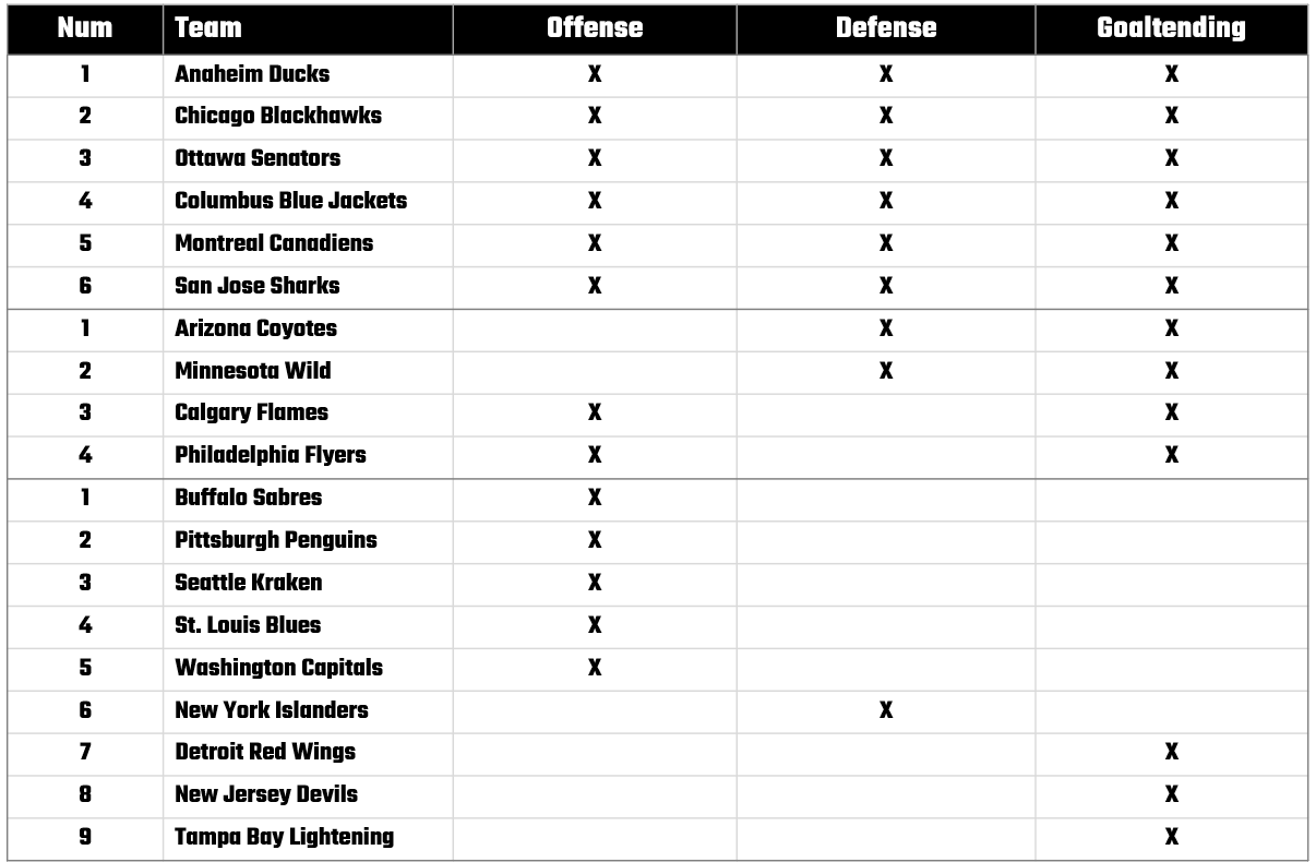
All told, according to our high-level analysis, nineteen teams are performing weaker in one or more of the offense, defense and goaltending areas and should be seeking help – for example, through incoming drafts, trades or pulling from their minor-league teams. For the purposes of this six-week series, we'll be mapping the incoming draft prospects to the teams that need the talent the most.

To watch a quick-hit video walkthrough, check out the YouTube video below.

Summary

This was the third week in our six-week newsletter series on Preparing for the NHL 2024 Draft. In this edition, we continued the analysis on the team stats, focusing on offense, defense and goaltending composite metrics. We created these composite metrics using raw and calculated statistics. We didn't use every hockey statistic, so you should think of this composite metric as directional and not comprehensive. (You should experiment with your own composite metrics to see if and how your results differ from ours.)

We ran three different analyses. The first was a trend analysis across three seasons using a PivotTable using Microsoft Excel. After we pivoted the offense, defense and goaltending data we then created a table with a sparkline trend and three-year average as a heatmap. We then sorted the views in descending order, so you could see those teams that ranked higher to lower. The second analysis was the ranking of offense, defense and goaltending scores with an associated quartile. This allowed us to categorize the lowest- to highest-performing teams. The final analysis was running a K-Means cluster analysis against one season's worth of data, so we could narrow the top, middle and bottom teams.

Using the K-Means cluster analysis as our grouping method, we then created a view that presented the teams with the highest need (they have needs across all three areas), then teams that have needs across two areas and then finally teams that have need in one area. We will come back to this view after we analyze the incoming draft prospects – we will map prospects to teams.

In next week's newsletter, we'll explore the incoming prospects by doing some data discovery and an exploratory data analysis on the top prospects.

Subscribe to our newsletter to get the latest and greatest content on all things hockey analytics!