Optimizing your Predictive Models

In this Edition
- AI Series: What We've Covered?
- What is Model Optimization?
- What are Optimization Methods?
- Optimizing a Predictive Model
AI Series: What We've Covered?
Our goal this summer was to spend more time on advanced topics, so by the time we hit the new hockey season, you have a good range of AI-related hockey analytics topics to use for your own learning and exploration.
To date, we've covered the following AI topics:
- Instant Hockey Analyses using ChatGPT and AI
- Using Linear Regression to Predict Goals
- Finding the Top Snipers using K-means Clustering
- Predicting Game Wins using Logistic Regression
- Predicting Wins using Support Vector Machine Models
- Driverless AI: Building the Perfect Predictive Model
In this week's newsletter, we'll introduce you to the concept of AI model optimization, different ways to do it and then demonstrate practical examples using a Support Vector Machine (SVM) model. The SVM optimization examples will use the classification model we built in a recent newsletter.
What is Model Optimization?
Simply put, model optimization is the process of improving the performance of your model. For example, if you build a multivariate Linear Regression model to predict team goal-scoring (let's say it's shots on goal, expected goals, faceoff percentage, and penalties), you might optimize the model by reducing the number of predictors (such as penalties) which should result in a stronger model. This process is called optimization.

Thus, model optimization is the process of improving the performance of a predictive model by implementing different techniques to achieve the best possible result. This involves a series of approaches and strategies to fine-tune the model to make it more accurate, efficient, and generalizable to new data. For example, you can adjust the hyperparameters for your model; create, select and transform features; apply regularization techniques; implement ensemble methods; and so on.
Let's take a closer look at some optimization methods.
What are Optimization Methods?
Optimizing an AI model involves various techniques that can enhance its performance and predictive accuracy. Below are examples of different optimization methods.
Data Preprocessing
This first area is about making sure your data has high integrity. For example, you optimize the model by making sure there are no missing values and use imputation techniques to fill in missing data appropriately. Also, identify and address outliers that could skew model training.
Feature Engineering
To optimize your model through feature engineering, you can remove irrelevant or redundant features to reduce dimensionality and improve model performance. That is, you simplify the model and then build, test and iteratively add more features to find where your model starts to degrade. You can also standardize or normalize features to ensure they have a similar scale. And lastly, you can create new features or transform existing ones to better capture underlying patterns in the data.
Hyperparameter Tuning
To optimize your model through hyperparameter configuration, you can systematically search through a predefined set of hyperparameters to find the optimal values. And you can use cross-validation techniques, for example, k-fold cross-validation to ensure the hyperparameters generalize well to new data.
Regularization
Regularization can also be used to optimize your models (to prevent overfitting) by adding a penalty to the model's complexity. Penalty parameters help control the trade-off between achieving a low training error and a low testing error.
Algorithm-Specific Tuning
To optimize using algorithm-specific tuning, you can experiment with different AI approaches and algorithms, explore different kernels (e.g., linear, polynomial, RBF) and kernel parameters (e.g., gamma in RBF kernel), and even experiment with ensemble methods such as bagging and boosting (combine multiple models to reduce variance and improve robustness).
Model Evaluation and Validation
Another way to optimize your models is to be consistent in your application of performance metrics such as accuracy, precision, and recall to evaluate and compare model performance. Further, you can include cross-validation within your optimization methods to ensure stability and robustness.

These are a few areas to start your optimization journey. As you engage more deeply with optimization within specific scenarios and algorithm types, you'll naturally find more ways to improve the performance of your AI models.
Optimizing a Predictive Model
In an earlier newsletter in this AI series, we built a predictive classification model (Win/Lose) using SVM. The predictive strength (i.e., the accuracy) for this model was 79%; however, we only took you to the step of creating, testing and visualizing the model. Below is the dataset and R code we used to build the SVM model.
This is fine for demonstrating how to build a model, but in a real-world scenario, you'd spend a lot of time optimizing your models (and then rebuilding, testing and optimizing your models at regular intervals to manage against model "drift") to make sure you get the best possible performance for your model.
From the last section, we introduced several different techniques to use when optimizing the model. When you're first starting out building predictive models, there are some simpler techniques that you can use (which are also cross-applicable to many different model types). For example, with the SVM model we built in our earlier newsletter, we could:
- Validate the integrity of the data. This is an easy way to make sure that there are no issues with your data that could ultimately skew the building of the model.
- Tune the hyperparameters of the model. This is a low-cost change that could allow us to see if a simple reconfiguration could improve the model.
- Add or remove features. Feature selection is a critical part of any model-building process, so tuning the features (or even creating new ones that may be more relevant to the model would be appropriate.
- Cross validate the model. By using a technique like k-fold cross-validation, we could better assess model performance.
Let's take two of the above optimization techniques and use the previously-built SVM model to explore whether we can improve the performance of the model. We'll walk through 1) tuning the hyperparameters and 2) exploring feature selection.
Tuning the Hyperparameters
One key hyperparameter in an SVM model is the type of kernel used in that model. The different kernels used in SVM-based models transform the input data into a higher-dimensional space where a linear separation is possible, even if the data is not linearly separable in the original space. Each kernel can impact the analysis in slightly different ways.
For example, the linear kernel is the simplest kernel function and is best suited for linearly separable data, where a straight line (or hyperplane in higher dimensions) can separate the classes. Thus, it provides a linear decision boundary, which may not capture the complexity in cases where the relationship between features and the target variable is non-linear.
The polynomial kernel represents the similarity of vectors in a polynomial feature space and is suitable for non-linear data where the relationship between the features and the target variable can be represented as a polynomial. The polynomial kernel introduces polynomial features, allowing for more complex decision boundaries.
The radial basis function (RBF) kernel is a popular non-linear kernel that measures the similarity between points based on their Euclidean distance. It is effective in situations where the relationship between the features and the target variable is highly non-linear. It also projects data into an infinite-dimensional space, allowing for very flexible decision boundaries.
Lastly, the sigmoid kernel, also known as the hyperbolic tangent kernel, is similar to the activation function used in neural networks. It is often used when the problem has similarities with neural network approaches.
Each kernel also carries a different practical consideration, three of which are listed below.
- Computational Cost: Linear kernels are computationally less expensive, while non-linear kernels like RBF and polynomial can be more computationally intensive.
- Model Complexity: Non-linear kernels can model complex relationships but also run the risk of overfitting, especially with high-dimensional data or small datasets.
- Parameter Tuning: Non-linear kernels often require careful tuning of their parameters (e.g., gamma for RBF, degree for polynomial) to achieve optimal performance.
Let's take the SVM model and re-run the model with the same features and examine the difference in their performance.
Linear
The first kernel we'll try is the linear kernel. We've included a subset of the code from the original SVM model and re-run the building of the SVM model, tested the model using the predict() function and created a confusion matrix to display the results.
svm_model_linear <- svm(WIN ~ ., data = data_train_df, type = 'C-classification', kernel = 'linear', probability = TRUE)
predictions_linear <- predict(svm_model_linear, newdata = data_test_df, probability = TRUE)
probabilities_linear <- attr(predictions_linear, "probabilities")

confusion_matrix_linear <- confusionMatrix(predictions_linear, data_test_df$WIN)
print(confusion_matrix_linear)
For the sake of brevity, we'll only include the accuracy result for the linear kernel, which was 0.7943 or 79.43%. We'll use this as our baseline.
Polynomial
The second kernel is the polynomial kernel and the code snippet below follows the same pattern as above.
svm_model_polynomial <- svm(WIN ~ ., data = data_train_df, type = 'C-classification', kernel = 'polynomial', degree = 3, probability = TRUE)
predictions_polynomial <- predict(svm_model_polynomial, newdata = data_test_df, probability = TRUE)
probabilities_polynomial <- attr(predictions_polynomial, "probabilities")

confusion_matrix_polynomial <- confusionMatrix(predictions_polynomial, data_test_df$WIN)
print(confusion_matrix_polynomial)
The result in this case is 0.8082 for accuracy or 80.82%, so a slight increase over our baseline.
Radial
The next kernel is the radial kernel, and again we follow a similar pattern to test this out in code.
svm_model_rbf <- svm(WIN ~ ., data = data_train_df, type = 'C-classification', kernel = 'radial', probability = TRUE)
predictions_rbf <- predict(svm_model_rbf, newdata = data_test_df, probability = TRUE)
probabilities_rbf <- attr(predictions_rbf, "probabilities")

confusion_matrix_rbf <- confusionMatrix(predictions_rbf, data_test_df$WIN)
print(confusion_matrix_rbf)
The result in this case is 0.7902 for accuracy or 79.02%, so a slight decrease from our baseline.
Sigmoid
And finally, the sigmoid kernel.
svm_model_sigmoid <- svm(WIN ~ ., data = data_train_df, type = 'C-classification', kernel = 'sigmoid', probability = TRUE)
predictions_sigmoid <- predict(svm_model_sigmoid, newdata = data_test_df, probability = TRUE)
probabilities_sigmoid <- attr(predictions_sigmoid, "probabilities")

confusion_matrix_sigmoid <- confusionMatrix(predictions_sigmoid, data_test_df$WIN)
print(confusion_matrix_sigmoid)
Interestingly, the model performance degrades here significantly, resulting in an accuracy of 0.6923 or 69.23%.
To better visualize the results, here's a bar chart that plots the accuracy of each kernel.
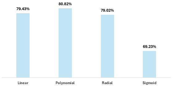
In sum, you can make a minute gain by optimizing for the kernel (specifically, the polynomial kernel), which is a relatively simple way to tune your models. Critical, though, is understanding what kernel would be appropriate for the shape and linearity of your data.
Let's move onto a second optimization example, which is feature selection.
Feature Selection
In AI and machine learning, features (aka attributes or variables) are the individual measurable properties or characteristics of the phenomena being observed. Features are the input variables that the AI model uses to make predictions or classifications.
In the original SVM model we built, the input variables we used were as follows:
- Shots For Percent (SF_PCT)
- Expected Goals Percent (XGF_PCT)
- Corsi For Percent (CF_PCT)
- Fenwick For Percent (FF_PCT)
- High Danger Goals For Percent (HDGF_PCT)
- Time on Ice (TOI)
- PDO Metric (PDO)
Optimizing feature selection means adding or removing features to the model. For hockey, this might be raw or calculated statistics or it might be your own custom feature. So, let's go ahead and test out removing features from this original dataset to see if this results in any differences in accuracy.
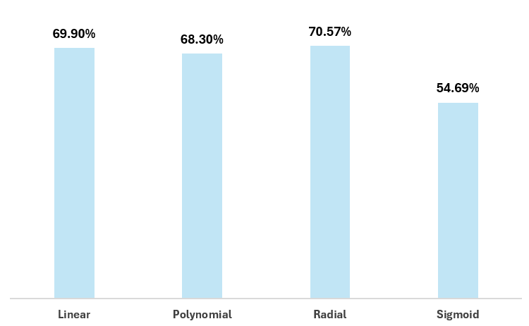
For example, let's trim the features to the following variables:
- SF_PCT
- XGF_PCT
- HDGF_PCT
If we re-run the models that test against each of the kernels, we see the accuracy shifts as follows.
Let's repeat the feature selection and this time edit the features to the following variables:
- SF_PCT
- XGF_PCT
- CF_PCT
- FF_PCT
- HDGF_PCT
Again, if we re-run the models that test against each of the kernels, we see the accuracy shifts as follows.
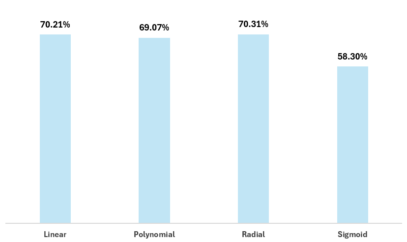
So, just with these two experiments where we edit the features from the original model, we see a concerted degradation of 9%+. Thus, if these were the only features available to us, we should revert back to the original set of features and go with the polynomial kernel to reach ~80% accuracy.
Summary
In this week's newsletter, we introduced you to the concept of model optimization, which is the process of applying different techniques to get to the best-performing AI model. We also introduced you to different optimization methods, ranging from data preprocessing, hyperparameter tuning, feature selection, and more.
We then walked through two examples of model optimization using an SVM model we built in a recent newsletter. The dataset and R code for this model can be found below:
We explored different kernel configurations in our AI model and then tested using different features within the model and compared the results. We found that the original features produced the best outcome, but with also a slight kernel re-configuration from linear to polynomial. This boosted our model from 79.07% to 80.82% – a modest increase from the original SVM accuracy.
Subscribe to our newsletter to get the latest and greatest content on all things hockey analytics!
Member discussion