Predicting Wins using Support Vector Machine Models

In this Edition

• AI Series: What We've Covered?
• What is Support Vector Machine?
• What are the Practical Applications of SVM?
• Walkthrough: Improving Model Performance using SVM

AI Series: What We've Covered?

Our goal this summer was to spend more time on advanced topics, so by the time we hit the new hockey season, you have a good range of AI-related hockey analytics topics to use for your own learning and exploration.

To date, we've covered the following AI topics:

• Instant Hockey Analyses using ChatGPT and AI
• Using Linear Regression to Predict Goals
• Finding the Top Snipers using K-means Clustering
• Predicting Game Wins using Logistic Regression

In this week's newsletter, we'll introduce you to the Support Vector Machine (SVM) model with the goal of improving on the predictive performance from the Logistic Regression model we implemented in our last newsletter.

What is Support Vector Machine?

Support Vector Machine (SVM) is a supervised machine learning algorithm used for classification and regression tasks. SVMs are known for their effectiveness in high-dimensional spaces and are used in scenarios where the number of dimensions exceeds the number of samples.

According to Brett Lantz, in Machine Learning with R:

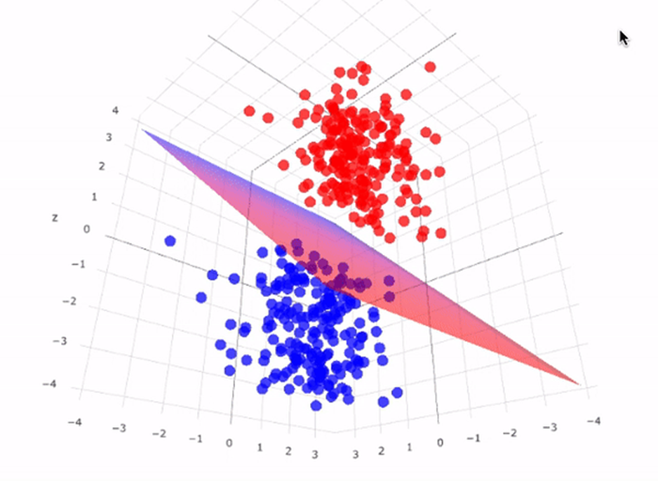
A support vector machine (SVM) can be imagined as a surface that creates a boundary between points of data plotted in a multidimensional space representing examples and their feature values. The goal of an SVM is to create a flat boundary called a hyperplane (p. 294).

This optimal hyperplane separates the data into different classes. For linearly separable data, this hyperplane is chosen to maximize the margin between the classes. For non-linearly separable data, SVM uses kernel functions to transform the data into a higher-dimensional space where a hyperplane can be used for separation.

In a recent article entitled Support Vector Machines (SVM): An Intuitive Explanation, the author characterizes (and illustrates) SVMs as follows:

Support Vector Machines (SVMs) are are widely used in various fields, including pattern recognition, image analysis, and natural language processing.

SVMs are also versatile; they can be adapted for use with nearly any type of learning task, including both classification and numeric prediction. Yet, SVMs are most easily understood when used for binary classification, which is how the method has traditionally been applied (Lantz, pp. 294-295).

The main components of a SVM are as follows:

• Hyperplane: A decision boundary that separates different classes.
• Support Vectors: Data points that are closest to the hyperplane and influence its position and orientation.
• Margin: The distance between the hyperplane and the nearest support vectors from either class. SVM aims to maximize this margin.

Further, SVM uses various kernel functions to handle non-linear relationships by mapping the input data into higher-dimensional spaces, such as Linear Kernel, Polynomial Kernel, Radial Basis Function (RBF) Kernel, and Sigmoid Kernel.

SVM vs Logistic Regression

In our last newsletter, we focused on a Logistic Regression model to build a binary classification model (Win/Lose). The model's predictive accuracy was about 70%, so in this newsletter we're both interested in how Logistic Regression is different from SVM and which approach performs better.

SVM and Logistic Regression are both supervised learning algorithms used for classification tasks (which means we need to have some labeled data to use for training the model), but they have some key differences in their approaches, objectives, and implementation.

At the highest level, the main goal of SVM is to find the optimal hyperplane that maximizes the margin between different classes. It focuses on finding the decision boundary that best separates the classes by maximizing the margin (the distance between the hyperplane and the closest data points of each class, called support vectors). Conversely, Logistic Regression aims to model the probability of a binary outcome by fitting a logistic function (sigmoid curve) to the data. It estimates the parameters (weights) that maximize the likelihood of observing the given data.

One key difference between SVM and Logistic Regression is their decision boundaries. That is, the decision boundary for SVM is a hyperplane that maximizes the margin between classes. For non-linearly separable data, SVM uses kernel functions to transform the data into a higher-dimensional space where a linear hyperplane can be used. For Logistic Regression, the decision boundary is a linear function of the input features. It is determined by the weights that maximize the likelihood of the observed data. Logistic Regression always produces a linear decision boundary in the input feature space.

This means that Logistic Regression is a good choice for use cases that are inherently linear; however, SVM can handle non-linear relationships using kernel functions (e.g., polynomial, radial basis function (RBF), sigmoid). Kernels allow SVM to transform the input space into a higher-dimensional space where a linear decision boundary can be applied. Thus, SVM is more flexible.

The output for SVM is typically a class label. The decision function can also provide a distance from the decision boundary, which can be interpreted as a confidence score. Logistic Regression outputs probabilities for each class. The class label is determined by applying a threshold (usually 0.5) to the predicted probabilities. For our Win/Lose scenario, the probability as an output of the model is useful because it can be consumed by other applications – for example, win probability metrics, betting scenarios and fantasy hockey reports.

In short, SVM is focused on finding the optimal hyperplane with maximum margin and can handle non-linear relationships using kernels. And Logistic Regression models the probability of a binary outcome using a logistic function, providing interpretable coefficients and a straightforward approach for linear relationships.

What are the Practical Applications of SVM?

SVM can be used in both general and hockey-specific scenarios. Some examples of the general application of SVM are as follows.

• Classifying documents into different categories, for example, email filtering, organizing news articles, and sentiment analysis of customer reviews.
• Recognizing objects within images or categorizing images into different classes, for example, handwritten digit recognition, facial recognition, and medical image analysis.
• Classifying genes, proteins, and other biological structures, for example, cancer classification, gene function prediction, and protein structure prediction.
• Predicting stock prices or classifying financial instruments, for example, credit risk assessment, fraud detection, and stock market prediction.
• Classifying customers into different groups based on their behaviors and preferences, for example, targeted marketing campaigns, and personalized recommendations.

Some examples of hockey-specific applications of SVM are as follows.

• Classifying players into different performance levels (e.g., Elite, Average, Below Average, etc.) based on their statistics such as goals, assists, and plus-minus ratings.
• Predicting the outcome of a game (Win/Loss) based on team statistics, player form, and other relevant metrics.
• Assessing the risk of injury for players based on their physical attributes, playing style, and historical injury data.
• Classifying teams or players into different play styles (e.g., defensive, offensive, balanced) based on game statistics.

Let's take another run at the Win/Loss prediction model we built using the Logistic Regression approach to see if using SVM offers anything different or improved.

Walkthrough: Improving Model Performance using SVM

There are two resource files that accompany this walkthrough, which you can download from the links below.

1. Hockey Stats (Game-Level) Dataset
2. R Code for the SVM Model

Before you start the walkthrough, create a local folder and download these files into that folder.

Hockey Stats for the SVM Model

If you remember, we built the Logistic Regression model using the following game statistics.

• Shots For Percentage (SF_PCT)
• Expected Goals For Percentage (XGF_PCT)
• Corsi For Percentage (CF_PCT)
• Fenwick For Percentage (FF_PCT)
• High Danger Goals For Percentage (HDGF_PCT)

For this walkthrough, we also added two more game stats:

• Time on Ice (TOI)
• PDO

These, more generally, had some correlation to wins, so we included them to see if they would augment the model.

Steps in the Walkthrough

The specific steps in this walkthrough include:

• Sourcing Data: Source and gather relevant data such as player stats, game results, and other performance metrics. (This will be a simple ingestion process given we've created a clean dataset for this walkthrough.)
• Model Training: Train the SVM model using the training data using an appropriate set of parameters.
• Model Evaluation: Evaluate the model's performance using metrics like accuracy, precision, recall, and so on.
• Model Visualization: Visualize the strength of the predictive model using a confusion matrix and ROC curve.

Let's get started!

Sourcing Data

We'll assume you've already downloaded the data and have it in a local folder. So, to get started, open RStudio and create a new project and use your existing directory (where you downloaded the data and our completed R code file).

The first step is to add a code section and include the various libraries you'll use in this walkthrough (or additional exploration you may want to do around SVM).

library(e1071)
library(ggplot2)
library(dplyr)
library(caret)
library(glmnet)
library(pROC)
library(tidyverse)
library(reshape2)
library(knitr)
library(kableExtra)
library(broom)

The next code snippet is to read the CSV file into an R data frame (game_data_df) and then select the specific columns you want to include in the SVM model. (Here is where you can trim or add statistics to include in the model.) And lastly, we set the WIN column as a factor.

game_data_df <- read.csv("svm_classification_game_data.csv")

game_data_df <- game_data_df %>% 
    select(WIN, SF_PCT, XGF_PCT, CF_PCT, FF_PCT, HDGF_PCT, TOI, PDO)

game_data_df$WIN <- as.factor(game_data_df$WIN)

With the data frame in R, you are now ready for the next step.

Model Training

You will now want to split your dataset into a training and test dataset. You do this to ensure a more optimal fit for your model. To do this, we first create an index that splits the data into 80% training data and 20% test data. We then use the svm() function to train the model using the training data (data_train_df).

set.seed(123)

train_index <- createDataPartition(game_data_df$WIN, p = .8, list = FALSE, times = 1)

data_train_df <- game_data_df[train_index,]
data_test_df  <- game_data_df[-train_index,]

data_test_df$WIN <- factor(data_test_df$WIN, levels = levels(data_train_df$WIN))

svm_model <- svm(WIN ~ ., data = data_train_df, type = 'C-classification', 
                kernel = 'radial', probability = TRUE)

You can optionally print out the SVM model (i.e., svm_model) to see the results if you want.

Model Evaluation

To evaluate the model, you'll want to use the test data (data_test_df) and apply the model to predict the results.

predictions <- predict(svm_model, data_test_df[, -1])

predictions <- factor(predictions, levels = levels(data_test_df$WIN))

confusion_matrix <- confusionMatrix(predictions, data_test_df$WIN)

The result of this is a confusion matrix that summarizes the performance of the SVM model.

Model Visualization

To visualize the confusion matrix, you can use the print() function, e.g., print(confusion_matrix), or you can choose to up-level your visualization. Given you may want to include this in a report, we've offered a visual rendering of the confusion matrix. To do this, we translate the confusion matrix into a data frame and then visualize it using ggplot.

conf_matrix_table <- as.table(confusion_matrix$table)

conf_matrix_df <- as.data.frame(conf_matrix_table)

ggplot(conf_matrix_df, aes(x = Prediction, y = Reference, fill = Freq)) +
  geom_tile() +
  geom_text(aes(label = Freq), color = "white", size = 6) +
  scale_fill_gradient(low = "blue", high = "orange") +
  labs(title = "Confusion Matrix", x = "Predicted", y = "Actual") +
  theme_minimal() +
  theme(axis.text.x = element_text(angle = 45, hjust = 1))
  

The result is a more aesthetic visualization that is easier to read.

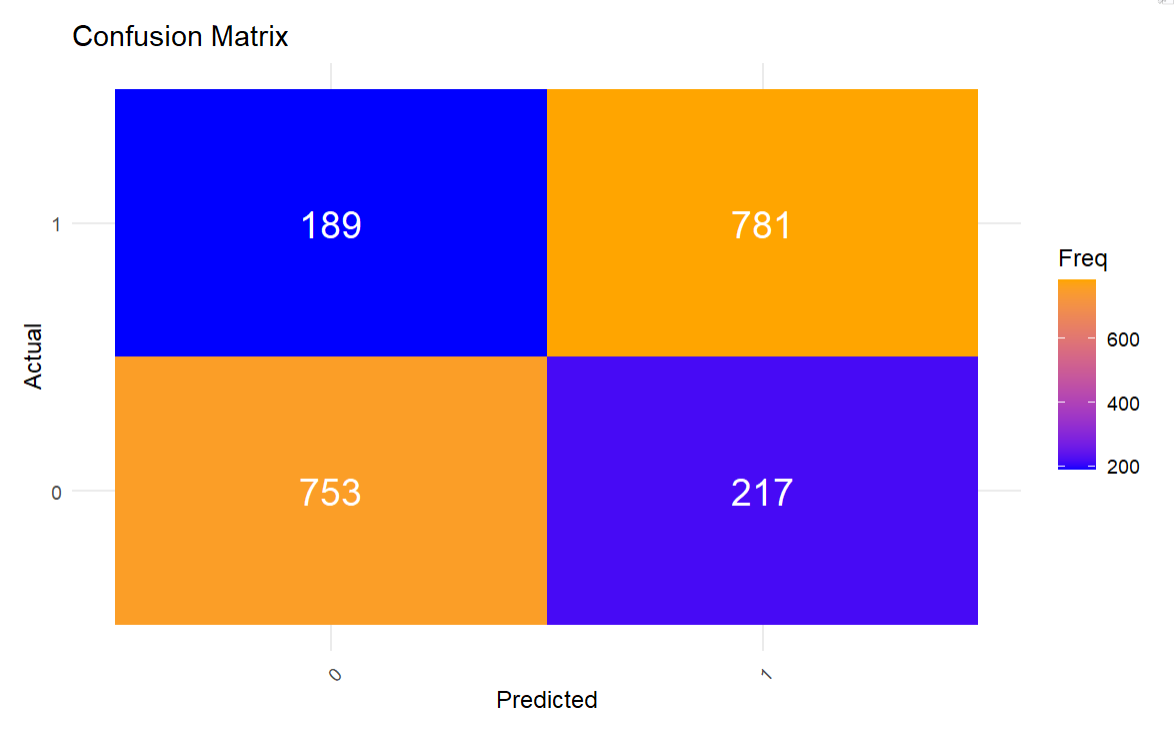
The way to read the above is as follows:

• True Negatives: The model correctly predicted 753 instances as class 0.
• False Negatives: The model incorrectly predicted 189 instances as class 0, which are actually class 1.
• False Positives: The model incorrectly predicted 217 instances as class 1, which are actually class 0.
• True Positives: The model correctly predicted 781 instances as class 1.

These are not the only metrics to extract from the SVM model results. We can also extract additional metrics around precision and recall to get a more quantified picture of the model performance. In the code below, we do some clean-up on the data objects and then use the kable() function to print out a more stylized table.

confMatrix_byClass <- as.data.frame(t(as.matrix(confusion_matrix$byClass)))

conf_by_class_df <- as.data.frame(confusion_matrix$byClass)
conf_by_class_df$METRICS = rownames(conf_by_class_df)
colnames(conf_by_class_df) <- c("VALUES", "METRICS")
rownames(conf_by_class_df) <- C(1:11)

con_by_class_matrix_df <- conf_by_class_df %>% 
  select(METRICS, VALUES)

con_by_class_matrix_df$VALUES <- round(con_by_class_matrix_df$VALUES, 4)

kable(con_by_class_matrix_df, format = "html", caption = "Statistics by Class") %>%
  kable_styling(bootstrap_options = c("striped", "hover", "condensed", "responsive"), 
                full_width = F) %>%
  column_spec(1, bold = FALSE, color = "black", background = "lightblue") %>%
  column_spec(2, bold = FALSE, color = "black", background = "orange")
  

Overall, the SVM model demonstrates solid performance with an accuracy of 79.07%, a balanced sensitivity (77.63%) and specificity (80.52%), and good precision (79.94%). The Kappa value indicates moderate agreement between predictions and actual outcomes. The model's performance is significantly better than random guessing, as indicated by the p-value for accuracy. The McNemar's test p-value suggests no significant difference between the rates of false positives and false negatives, indicating balanced performance in identifying both classes. The balanced accuracy aligns with the overall accuracy, showing the model's robustness in handling both positive and negative classes.

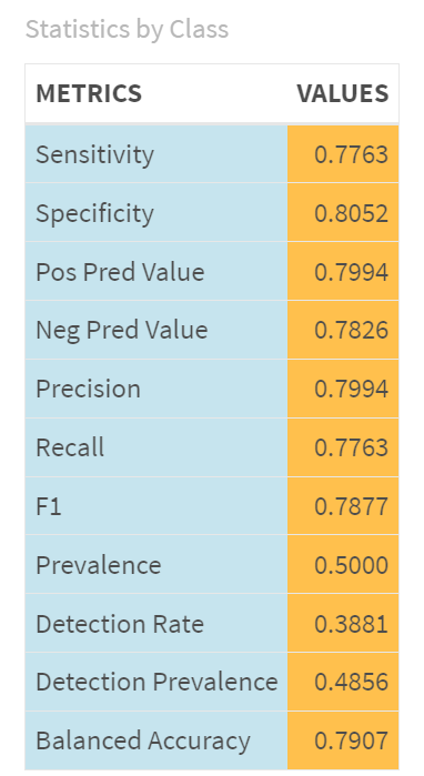
If we compare the performance of this SVM model to our Logistic Regression model, we find an overall 9% improvement in the performance of the SVM model. It bears repeating that we did add a couple of features of the SVM model, but that notwithstanding the model did improve.

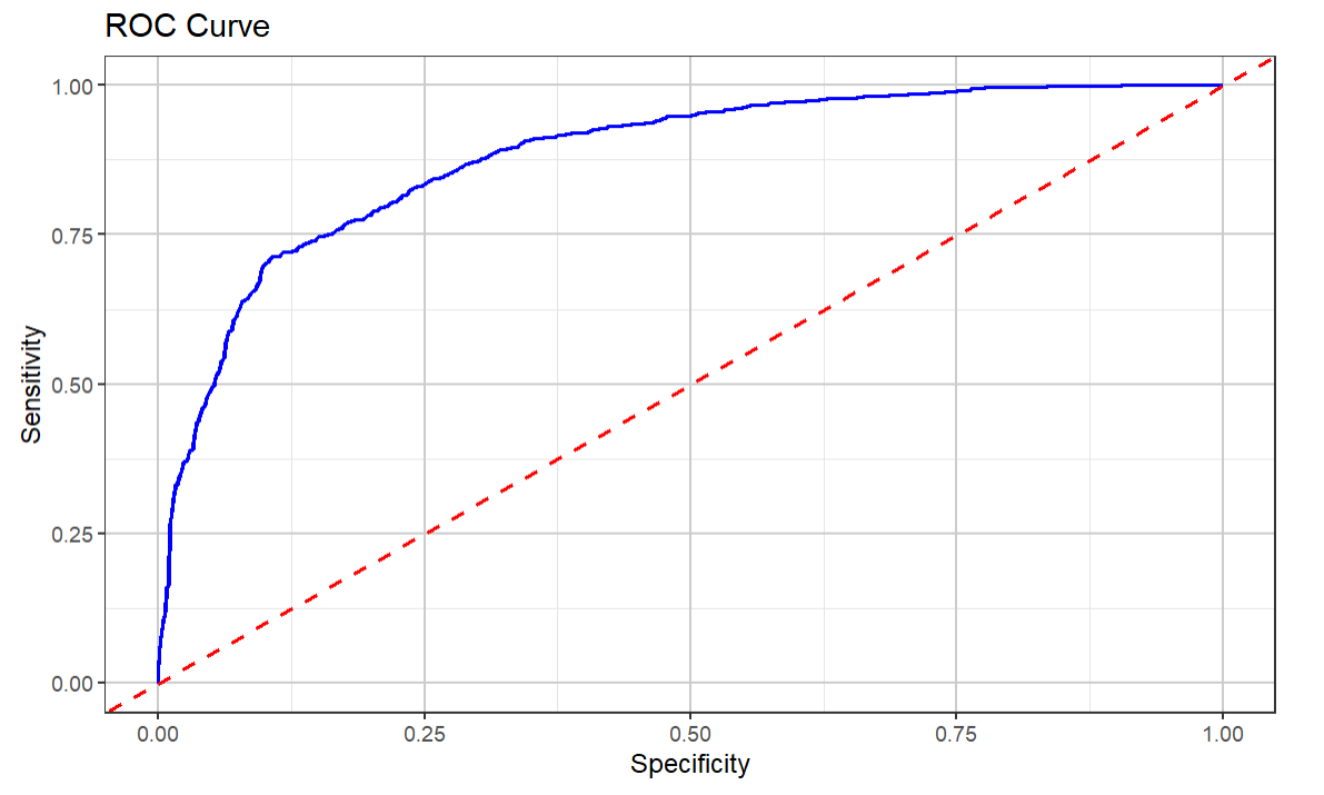
The final visualization is the ROC (Receiver Operating Characteristic) curve, which is a graphical representation of a classification model's performance across different threshold values. It plots the True Positive Rate (Sensitivity) against the False Positive Rate (1 - Specificity) at various threshold settings. The ROC curve is used to visualize and evaluate the trade-offs between the benefits (true positives) and costs (false positives) of a classification model.

The code snippet below creates a separate predictions and probabilities vector and uses the roc() function to plot the ROC curve.

predictions_2 <- predict(svm_model, data_test_df[, -1], probability = TRUE)  
probabilities_2 <- attr(predictions_2, "probabilities")[,2]

roc_obj <- roc(data_test_df$WIN, probabilities_2)

roc_data <- data.frame(
  specificity = roc_obj$specificities,
  sensitivity = roc_obj$sensitivities
)

ggplot(roc_data, aes(x = 1 - specificity, y = sensitivity)) +
  geom_line(color = "blue",  size = .75) +
  geom_abline(linetype = "dashed", color = "red", size = .75) +
  theme_bw() + 
    labs(
    title = "ROC Curve",
    x = "Specificity",
    y = "Sensitivity"
  ) +
  theme_bw() + 
  theme(
    panel.grid.major = element_line(color = "grey80"), 
    panel.grid.minor = element_line(color = "grey90") 
  )

You can see that the resulting ROC curve is closer to the top-left portion of the visualization, and this indicates a more performant model. Further, the Area Under the Curve (AUC) is higher, which also indicates a better model performance.

This reinforces the performance of the SVM model and the fact that is a better model that our previous Logistic Regression model.

Check out our quick-hit video on YouTube below.

Additional Methods to Optimize Your Predictive Models

We favor testing and re-testing models until you find an optimal and consistent performance in your predictive models. Note that you're not limited to just Logistic Regression and SVM models when it comes to predicting wins. You can also continue to optimize the performance of your model using, for example, ensemble methods.

Ensemble methods are techniques that combine multiple models to improve the overall predictive performance compared to individual models. The key idea is that by combining different models, the ensemble can leverage the strengths of each model and mitigate their weaknesses, leading to better generalization and robustness. Some common ensemble methods are:

• Bagging - training multiple models independently on different random subsets of the training data and then averaging their predictions (for regression) or taking a majority vote (for classification). Random Forests are an example.
• Boosting - trains models sequentially, where each model tries to correct the errors of the previous model. The final prediction is a weighted sum of the predictions of all models. Gradient Boosting Model and XGBoost are examples.
• Stacking - training multiple models (called base learners) and then training a meta-model to combine their predictions. The meta-model learns how to best combine the base models' predictions.
• Voting - combines the predictions of multiple models by taking the majority vote (for classification) or averaging the predictions (for regression).

Point being: you have many different ways to optimize the model before you deploy into production.

Summary

In this week's newsletter, we introduced you to the Support Vector Machine (SVM) model, which is a form of supervised learning that can be used for both classification and regression models. We covered some general applications of the SVM model and some applications that are specific to hockey. We then walked through a demonstration of how to build and train an SVM model – using the same data we used to train a Logistic Regression model from our last newsletter.

The links for the resources for the walkthrough are below:

1. Hockey Stats (Game-Level) Dataset
2. R Code for the SVM Model

The result was that the SVM model performed 9% better at 79% – notwithstanding the addition of two features within the model. This was a positive optimization, but we'd recommend continuing to test different combinations of features (i.e., adding or removing hockey statistics from the model), tuning the parameters of the model or even using some of the ensemble methods mentioned at the end of the walkthrough.

In our next newsletter, we'll explore AutoML, which is a growing area in AI that automatically finds the best-performing model for you.

Subscribe to our newsletter to get the latest and greatest content on all things hockey analytics!