Predicting Wins using k-Nearest Neighbors
In this Edition
- AI Series: What We've Covered?
- What is k-Nearest Neighbors?
- What are Practical Uses for KNN?
- Walkthrough: Predicting Wins using KNN
AI Series: What We've Covered?
Our goal this summer was to spend more time on advanced topics, so by the time we hit the new hockey season, you have a good range of AI-related hockey analytics topics to use for your own learning and exploration.
To date, we've covered the following AI topics:
- Instant Hockey Analyses using ChatGPT and AI
- Using Linear Regression to Predict Goals
- Finding the Top Snipers using k-means Clustering
- Predicting Game Wins using Logistic Regression
- Predicting Wins using Support Vector Machine Models
- Driverless AI: Building the Perfect Predictive Model
- Optimizing your Predictive Models
In this week's newsletter, we'll introduce you to the concept of k-Nearest Neighbors, or KNN, which is a type of algorithm that can be used for classification and regression scenarios. We'll both introduce you to KNN and then walk through an example, which will continue the example of win predictions, testing whether KNN can improve on our previous algorithms.
What is k-Nearest Neighbors?
KNN is a simple, instance-based learning AI algorithm that you can use for classification and regression tasks. Instance-based learning is where a model stores all instances and makes decisions based on the proximity of new instances to those in the training set. For us, it was one of the first algorithms we learned (using it for classification use cases) as it's easy to use and a widely-adopted supervised learning technique.
If you've ever heard the expression "birds of a feather flock together," you'll get the basic gist of KNN. According to Brett Lantz (author of Machine Learning with R), "things that are alike tend to have properties that are alike." KNN implements this principle by classifying "data by placing it in the same category as similar or 'nearest' neighbors." Lantz offers the following:
The KNN algorithm gets its name from the fact that it uses information about an example's k nearest neighbors to classify examples. The letter k is a variable implying that any number of nearest neighbors could be used. After choosing k the algorithm requires a training dataset made up of examples that have been classified in several categories, as labeled by a nominal variable (p. 85).
Antony Christopher, in his article entitled K-Nearest Neighbor, does a great job illustrating the KNN algorithm through four easy-to-follow steps.
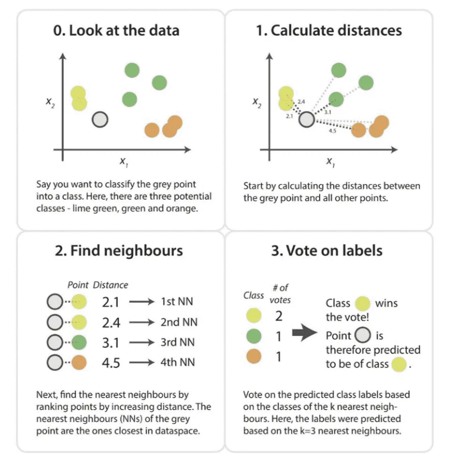
Thus, for classification models, KNN assigns a class to a new instance based on the majority class of its k-nearest neighbors. For regression, KNN predicts the value of a new instance based on the average of the values of its k-nearest neighbors. KNN typically uses Euclidean distance to measure similarity between instances, but other distance metrics like Manhattan, Minkowski, or Hamming distance can also be used.
How is KNN Different to Other Classification Techniques
KNN is a popular classification technique, but its suitability compared to other classification methods depends on the specific context and requirements of the application. Below is a comparison of KNN with other classification techniques.
Logistic Regression
The strengths of Logistic Regression are it's simple to implement, has interpretable coefficients, and works well for linearly separable data. We've used Logistic Regression in many different hockey use cases. However, the Logistic Regression model assumes linearity, so it can struggle with complex relationships or non-linear data. Compared to Logistic Regression, KNN may be a better choice especially where your scenario may have more non-linearity to it. Note, though, that with larger datasets KNN can sometimes be slower.
Decision Trees and Random Forests
The strengths of Decision Trees and Random Forest algorithms are they handle both linear and non-linear relationships, are interpretable, and handle missing values well. However, they can also overfit (e.g., Decision Trees), are more complex and can be resource-intensive (Random Forests). Interestingly, Random Forests generally outperform KNN in terms of accuracy and robustness, especially for complex datasets. And while KNN is simpler, it can be less effective for high-dimensional data.
Support Vector Machines (SVM)
SVM is effective in high-dimensional spaces and manages well against overfitting (with the appropriate kernel choice). However, SVM is also computationally intensive, less interpretable, and sensitive to parameter tuning. Compared to KNN, SVM often provides higher accuracy and better performance in complex, high-dimensional spaces. And again, while KNN is simpler, it can be less effective for high-dimensional data.
Neural Networks
The strengths of Neural Networks are that they can model complex patterns, are highly flexible, and state-of-the-art for many tasks. Its weaknesses are that it requires large datasets, is computationally expensive, and is harder to interpret. Neural Networks usually outperform KNN on large, complex datasets but at the cost of interpretability and computational resources. Note that KNN is easier to implement and understand.
Strengths and Weaknesses of KNN for Hockey Scenarios
The strengths of KNN are as follows:
- KNN is easy to understand and implement, making it accessible for various applications.
- It can handle non-linear relationships between features, which is useful for the complex nature of hockey data.
- KNN does not make strong assumptions about the data distribution, making it flexible for different types of hockey statistics.
- Results are straightforward to explain – predictions are based on the majority class of nearest neighbors.
The weaknesses of KNN are as follows:
- KNN can be slow with large datasets, as it requires computing distances for each query point.
- Performance degrades with high-dimensional data due to the curse of dimensionality, which is often a concern with sports data.
- KNN is sensitive to the scale of features, requiring careful preprocessing (e.g., normalization).
- It may struggle with imbalanced datasets, common in hockey where certain outcomes (e.g., wins) may be less frequent.
Let's look at some of the practical uses for KNN.
What are Practical Uses for KNN?
You can use KNN across several non-hockey use cases. For example: building classification models for handwriting recognition, image classification and document classification; building regression models for predicting house prices or estimating the amount of rainfall; building recommendation systems that suggest products to users based on the preferences of similar users; and anomaly detection such as identifying outliers or abnormal instances in a dataset, such as fraudulent transactions.
Central to this newsletter series, you can also use KNN for different hockey use cases. For example: player performance classification to categorize different skill levels and position suitability; predicting game outcomes, such as win/loss; classifying player similarity, such as finding players similar to a given player based on various performance metrics; and injury risk assessment, such as predicting the likelihood of a player getting injured.
Depending on the specific hockey scenario, you'll find KNN can be more or less useful. Scenarios better suited to KNN are as follows:
- Identifying similar players based on performance metrics.
- Predicting the outcome of games using historical data.
- Assessing the risk of player injuries based on past data.
Scenarios less suited for KNN are as follows:
- Real-time predictions, due to its computational intensity.
- Scenarios with high-dimensional data – methods like Random Forests or Neural Networks may perform better.
- For very large datasets, KNN may under-perform, so more scalable methods like gradient boosting or neural networks might be preferred.
In short, KNN is a versatile algorithm that is effective for certain hockey scenarios, especially those involving moderate-sized datasets and non-linear relationships. However, for high-dimensional, large-scale, or real-time applications, other methods like Random Forests, SVMs, or Neural Networks are often more suitable. The choice of algorithm should consider the specific requirements of the task, including interpretability, scalability, and computational resources.
Walkthrough: Predicting Wins using KNN
In our walkthrough, we'll replicate the classification of the outcome of a game (Win/Loss) to see how KNN performs against the other techniques we've used in this AI series.
For this walkthrough, we've published two resources that you can use to practice alongside the code in this walkthrough section. They are:
Download these files into a local folder, and then open RStudio.
The first code snippet are the libraries that we will use in the R application.
library(class)
library(caret)
library(ggplot2)
library(dplyr)
library(tidyverse)
library(reshape2)
library(knitr)
library(kableExtra)
library(broom)
The second code snippet is where we loaded the game stats data and then created a subset of the data.
data <- read.csv("knn_game_data.csv")
data_selected <- data[, c("WIN", "GF", "GA", "SF_PCT", "X_GF", "X_GA", "XGF_PCT",
                          "CF_PCT", "FF_PCT", "SCF_PCT", "HDSF_PCT",
                          "HDGF_PCT", "TOI", "PDO")]
We next recast the WIN column as a factor and then created a training and test set. As you likely know by now, the training set is used to train the KNN model, and the test set is used to test the predictive strength of the model.
data_selected$WIN <- as.factor(data_selected$WIN)

set.seed(123)
trainIndex <- createDataPartition(data_selected$WIN, p = 0.8, list = FALSE)
trainData <- data_selected[trainIndex, ]
testData <- data_selected[-trainIndex, ]

train_x <- trainData[, -1]
train_y <- trainData$WIN

test_x <- testData[, -1]
test_y <- testData$WIN
The next step is to build the KNN model, which is a simple process of setting the number of k nearest neighbors and building the model. Here we also create a confusion matrix to see the results of the model.
k <- 5
knn_pred <- knn(train = train_x, test = test_x, cl = train_y, k = k)
confusionMatrix(knn_pred, test_y)
Because the default confusion matrix is not super aesthetic, we create a better-looking version with the code snippet below. To do this, we create a table object (conf_matrix_table), transpose that to a data frame (conf_matrix_df) and use the ggplot() function to create a decent-looking confusion matrix.
conf_matrix_table <- as.table(confusion_matrix$table)
conf_matrix_df <- as.data.frame(conf_matrix_table)

ggplot(conf_matrix_df, aes(x = Prediction, y = Reference, fill = Freq)) +
  geom_tile() +
  geom_text(aes(label = Freq), color = "white", size = 6) +
  scale_fill_gradient(low = "blue", high = "orange") +
  labs(title = "Confusion Matrix", x = "Predicted", y = "Actual") +
  theme_minimal() +
  theme(axis.text.x = element_text(angle = 45, hjust = 1))
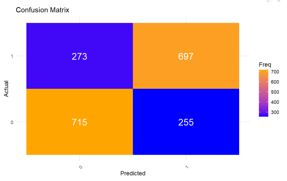
This results in the following confusion matrix. This looks to be a decent-performing model, but let's get at the model details to verify this observation.
The next code snippet creates a view with a set of metrics and values, which provide more information about the predictive strength of the KNN model. To do this, we parse out the statistics that we need and shape them in the form of a two-columned data frame (con_df) comprising the metrics and their respective values. We then do some clean-up on the values and create a more aesthetic table (using the ktable() function) that is easier and more intuitive to view.
con_df <- as.data.frame(confusion_matrix$overall)
con_df$METRICS = rownames(con_df)
colnames(con_df) <- c("VALUES", "METRICS")
rownames(con_df) <- C(1:7)

con_matrix_df <- con_df %>%
  select(METRICS, VALUES)

con_matrix_df$VALUES <- format(con_matrix_df$VALUES, scientific = FALSE, digits = 4)
con_matrix_df$VALUES <- as.numeric(con_matrix_df$VALUES)
con_matrix_df$VALUES <- round(con_matrix_df$VALUES, 4)

kable(con_matrix_df, format = "html", caption = "Overall Statistics") %>%
  kable_styling(bootstrap_options = c("striped", "hover", "condensed", "responsive"),
                full_width = F) %>%
  column_spec(1, bold = FALSE, color = "black", background = "lightblue") %>%
  column_spec(2, bold = FALSE, color = "black", background = "orange")
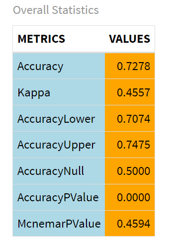
The key metric we want first is the overall accuracy of the KNN model, which as you can see is 0.7278 or 72.78%.
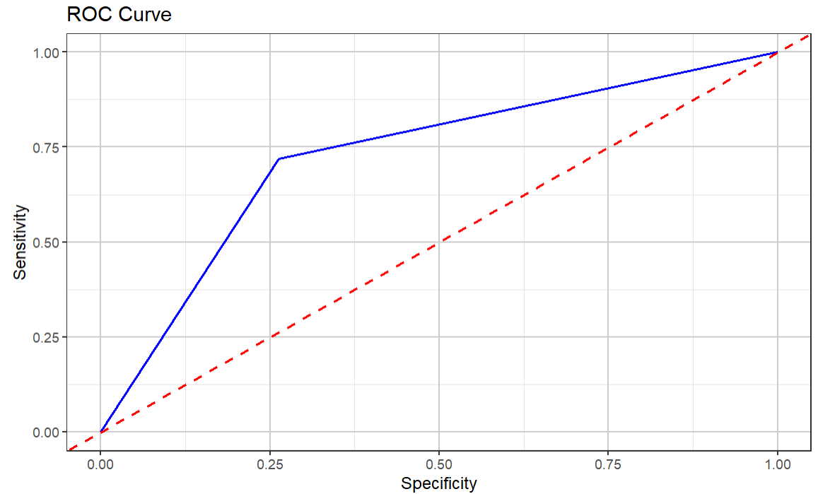
The final code snippet then plots an ROC curve so we can visualize the area under the curve (or AUC) to see how the sensitivity of the model compares against the specificity of the model.
roc_curve <- roc(test_y, as.numeric(knn_pred))

roc_data <- data.frame(
  specificity = roc_curve$specificities,
  sensitivity = roc_curve$sensitivities
)

ggplot(roc_data, aes(x = 1 - specificity, y = sensitivity)) +
  geom_line(color = "blue",  size = .75) +
  geom_abline(linetype = "dashed", color = "red", size = .75) +
  theme_bw() +
    labs(
    title = "ROC Curve",
    x = "Specificity",
    y = "Sensitivity"
  ) +
  theme_bw() +
  theme(
    panel.grid.major = element_line(color = "grey80"),
    panel.grid.minor = element_line(color = "grey90")
  )
The ROC curve shows that, again, the model is somewhat decent, but we'd want to keep trying different combinations or optimizations to see if we can improve the predictive strength of the model.
Comparing KNN to Other Approaches
In our AI and hockey analytics newsletter series, we've tested several different algorithms to predict wins/losses. While our main goal was to introduce you to different AI models and show you how to use them (and when to use them), we also wanted to see which one would perform the best. Out of all the approaches we tried, here are the different approaches and their respective accuracy scores.
- AutoML (H2O.ai): 99.99%
- SVM (Polynomial Kernel): 80.82%
- KNN: 72.78%
- Logistic Regression: 70.05%
Now of course you'd want to test, optimize and tune your models (especially with high-scoring models), but on its face, the AutoML approach (which was an ensemble model) was the best-performing approach.
Summary
In this newsletter, we introduced you to the concept of KNN, a simple, instance-based learning algorithm used for classification and regression tasks in machine learning. We also introduced you to different use cases where you could apply it, compared KNN to other approaches and enumerated different hockey scenarios where you might use KNN.
We also walked through an example – similar to our other newsletters – where we built a classification model to predict wins. Using KNN, we found the model resulted in a 72.78% accuracy rate, so not a terrible model. As a reminder, here are the resources for the walkthrough:
And while 72.78% is a decent-performing model, it was outperformed by the AutoML ensemble model (99.99%) and the SVM model (80.82%).
Subscribe to our newsletter to get the latest and greatest content on all things hockey analytics!
Member discussion