Predicting Game Wins using Logistic Regression

In this Edition

• AI Series: What We've Covered?
• What is Logistic Regression?
• What are the Practical Applications of Logistic Regression?
• Walkthrough: Using Game Statistics to Predict Wins

AI Series: What We've Covered?

Our goal this summer was to spend more time on advanced topics, so by the time we hit the new hockey season, you have a good range of AI-related hockey analytics topics to use for your own learning and exploration.

To date, we've covered the following AI topics:

• Instant Hockey Analyses using ChatGPT and AI
• Using Linear Regression to Predict Goals
• Finding the Top Snipers using K-means Clustering

In this week's newsletter, we'll introduce you to the Logistic Regression model and show you how you can use it to predict wins.

What is Logistic Regression?

Logistic regression is a statistical method used for binary classification problems, where the goal is to predict one of two possible outcomes based on one or more predictor variables. It models the probability that a given input point belongs to a certain class. According to Brett Lantz, author of Machine Learning in R, "the logistic function has the convenient property that for any input x value, the output is a value in the range between 0 and 1 – exactly the same range as a probability" (p. 217). A higher probability outcome implies a better level of predictability with the model.

The logistic regression model uses the logistic function, also known as the sigmoid function, to map predicted values to probabilities:

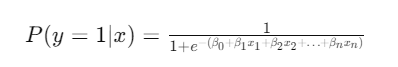
where:

• P(y=1∣x) is the probability of the event occurring.
• β0​ is the intercept.
• β1​,β2​,…,βn​ are the coefficients of the predictor variables x1, x2,…, xn.

There are various approaches when implementing a logistic regression model. For example: a Binary Logistic Regression is used when the outcome is binary (e.g., success/failure, yes/no); a Multinomial Logistic Regression is an extension of the binary logistic regression and is used when there are more than two classes; and the Ordinal Logistic Regression is used when the outcome has a natural order (e.g., rating scales).

Differences across Classification Techniques

When evaluating Logistic Regression with other classification algorithms, it's useful to understand the differences across them. For example, to follow are some of the differences between Logistic Regression and other classification techniques.

Linear vs. Non-Linear Decision Boundaries

Logistic regression provides a linear decision boundary. Algorithms like Support Vector Machines (SVM) with non-linear kernels, Decision Trees, and Neural Networks can provide non-linear decision boundaries.

Model Interpretability

Logistic Regression is highly interpretable as the coefficients indicate the direction and magnitude of the relationship between predictors and the outcome. Models like Random Forests, Gradient Boosting, and Neural Networks are often considered less interpretable.

Assumptions

Logistic Regression assumes a linear relationship between the log-odds of the outcome and the predictor variables. Other algorithms like Decision Trees and k-Nearest Neighbors (k-NN) make fewer assumptions about the data structure.

Handling of Multicollinearity

Logistic Regression can be sensitive to multicollinearity among predictors, requiring techniques like regularization (L1 or L2) to handle it. Tree-based methods and ensemble methods are more robust to multicollinearity.

Let's now look at both general applications of Logistic Regression as well as those that apply to hockey.

What are Practical Applications of Logistic Regression?

In this section, we'll detail both general applications of Logistic Regression and those that are specific to hockey.

General Applications of Logistic Regression

Medical Diagnosis

Predicting the presence or absence of a disease based on patient data. For example, predicting the likelihood of heart disease based on patient characteristics and test results.

Marketing

Predicting customer responses to marketing campaigns. For example, predicting whether a customer will purchase a product based on demographic and behavioral data.

Credit Scoring

Assessing the likelihood of a loan applicant defaulting on a loan. For example, predicting loan default based on credit history, income, and other financial indicators.

Fraud Detection

Identifying fraudulent transactions based on transaction characteristics. For example, predicting whether a transaction is fraudulent based on transaction amount, location, and time.

Risk Management

Estimating and managing risks in various domains such as finance, insurance, and operations. For example, predicting the risk of insurance claims based on policyholder data.

E-commerce

Predicting customer behavior and optimizing sales strategies. For example, predicting customer churn based on usage patterns and interaction history.

Practical Applications of Logistic Regression for Hockey

To follow are several examples of where you can use Logistic Regression in hockey analytics.

Win Probability Prediction

Predicting the probability of a team winning a game based on various game factors (e.g., shots on goal, faceoff wins, penalties, and power plays). For example, live win probability updates during games or a pre-game analysis to estimate the likelihood of victory against opponents.

Player Performance Evaluation

Assessing whether a player will score a goal in a given game or period based on their historical performance, position, time on ice, and situational factors (e.g., power play, penalty kill). For example, scouting and player evaluations, identifying players likely to score under specific conditions.

Injury Risk Assessment

Predicting the likelihood of a player getting injured based on factors such as age, minutes played, physical play style, and historical injury data. For example, managing player workload, developing preventive measures, and strategizing player rotations.

Goalie Performance Analysis

Estimating the probability of a goalie making a save given certain shot characteristics (e.g., shot distance, angle, and shot type). For example, evaluating goalie performance, identifying areas for improvement, and comparing goalie performance under different conditions.

Special Teams Effectiveness

Predicting the success rate of power plays and penalty kills based on team and player statistics, historical data, and situational variables. For example, optimizing special teams strategies, coaching decisions during games, and pre-game planning.

Player Development and Scouting

Predicting the future success of young players or draft picks based on junior league performance, physical attributes, and psychological assessments. For example, draft decision-making, player development planning, and long-term team building.

Fan Engagement and Betting Markets

Creating models to predict game outcomes, player performance, or in-game events (e.g., first goal scorer) to engage fans and inform betting markets. For example, enhancing fan experience through interactive tools, supporting fantasy hockey, and providing data for sports betting.

Lineup Optimization

Predicting the optimal line combinations or defensive pairings that maximize the team's chances of winning based on player chemistry, performance metrics, and matchup data. For example, pre-game lineup decisions, in-game adjustments, and strategic planning.

Let's take the use case of predicting wins and walk through how to create a Logistic Regression model.

Walkthrough: Using Game Statistics to Predict Wins

In this walkthrough, we'll create a Logistic Regression model and test the predictive strength of the model. We'll use R and RStudio to code the model and select a small set of inputs for the model. The walkthrough will follow six steps:

1. Download the dataset and code and to a local directory.
2. Create a new R project and markdown file.
3. Load the dataset into a data frame and clean and transform the data.
4. Create a Logistic Regression model (using several input variables).
5. Test the predictive value of the Logistic Regression model.
6. Plot the ROC curve, which will show the relative strength of the model.

Download Dataset and R Code

We've prepared a dataset that you can use for your own experimentation with logistic regression (and other techniques) and also have created an R code sample file that you can also use to implement the Logistic Regression model. Below are the links to download the code and dataset.

• Multi-season Team Statistics Dataset
• R Code - Logistic Regression Analysis to Predict Wins

Create a New R Project and Markdown File

Create a local folder for the above files, and download them into that folder. Then, open RStudio and create a new project (using an existing folder – the folder you just created), name the project and then add the above R code file to that project.

The logistic regression model we'll build in this walkthrough is a multivariate logistic regression, meaning there are several independent variables acting as inputs into the model. They are:

• Shots For Percentage (SF_PCT)
• Expected Goals For Percentage (XGF_PCT)
• Corsi For Percentage (CF_PCT)
• Fenwick For Percentage (FF_PCT)
• High Danger Goals For Percentage (HDGF_PCT)

Because a win in hockey requires one team to score more goals than the other, we selected the above because they all in some way contribute to goals being scored. Also, note that the dataset is at the game level; that is, each row in the dataset represents a single game.

Load the Dataset into R and Transform the Data

The first code snippet are the libraries we'll use in the implementation of the logistic regression. There are more here than you might usually see in a small implementation script because we wanted to improve on the look and feel of the plots and matrices.

library(ggplot2)
library(dplyr)
library(caret)
library(glmnet)
library(pROC)
library(tidyverse)
library(reshape2)
library(knitr)
library(kableExtra)
library(broom)

The next code snippet reads the CSV file into a data frame (final_log_reg_df), creates a subset of the data, cleans and transforms the data. Note that our original dataset is an amalgamation of data we've sourced from the Internet and our own data provider, so there are different column heading cases that we want to make more consistent. Also, in one of the columns (HDGF_PCT) there are extraneous dashes that we want to convert to a value of 0, so all values are numeric. And lastly, we want to make sure that we remove all NAs from the data frame.

final_log_reg_df <- read.csv("final_log_regression_game_data.csv")

sub_final_log_reg_df <- final_log_reg_df %>% 
  select(Date, Team, Win, GF, GA, SF_PCT, xGF, xGA, xGF_PCT, CF_PCT, FF_PCT, SCF_PCT, HDSF_PCT,
         HDGF_PCT)

colnames(sub_final_log_reg_df) <- c("DATE", "TEAM", "WIN", "GF", "GA", 
                                    "SF_PCT", "X_GF", "X_GA", "XGF_PCT", 
                                    "CF_PCT", "FF_PCT", "SCF_PCT", "HDSF_PCT",
                                    "HDGF_PCT")

sub_final_log_reg_df <- sub_final_log_reg_df %>%
  mutate(HDGF_PCT = ifelse(HDGF_PCT == "-", 0, as.numeric(HDGF_PCT)))

na.omit(sub_final_log_reg_df)

With the data now clean and transformed, you are now ready to create the model.

Create a Logistic Regression Model

To avoid over- or under-fitting your model, it's important to create a training dataset and a test dataset – you don't train and test your model on the same data sample. After your data is cleaned and transformed, this is typically the next step. You use the training dataset to train the logistic regression model, and you then test the predictions that are being modeled against the test dataset. The below code snippet divides the original data into 80% for the training dataset and the remaining 20% for the test dataset.

set.seed(123)

train_index <- createDataPartition(sub_final_log_reg_df$WIN, p = .8, list = FALSE)

data_train_df <- sub_final_log_reg_df[train_index, ]
data_test_df <- sub_final_log_reg_df[-train_index, ]

The next code snippet builds a GLM model using a subset of the hockey statistics. It then visualizes the results of the modeling process. Note that we're building the model using the training set (data_train_df).

model <- glm(WIN ~ SF_PCT + XGF_PCT + CF_PCT + FF_PCT + HDGF_PCT, 
             data = data_train_df, family = binomial)

tidy_model <- tidy(model)

tidy_model %>%
  kable(format = "html", caption = "Logistic Regression Model Results") %>%
  kable_styling(bootstrap_options = c("striped", "hover", "condensed", "responsive"), full_width = F) %>%
  column_spec(1, bold = TRUE, color = "white", background = "dodgerblue") %>%
  column_spec(2:5, color = "black", background = "lightgray")
  

Below is the result of the logistic regression model using the five calculated hockey statistics. The p value is important here because if the input variable is not significant to the model below a certain threshold, then that variable doesn't help the model. For example, in the below table, you can see that the FF_PCT (Fenwick For Percentage) is not within the margin of significance (0.01 to 0.05), so it won't contribute to the model. You might consider removing input variables that don't "optimize" or contribute to the predictive strength of your model.

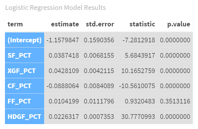
Given our goal was to use these input variables as a way to predict a win, let's do a quick check to see how each variable factors into the Logistic Regression model.

The Intercept (-1.158) value tells us the log-odds of winning when all other factors are zero. Since this is a negative number, it suggests that the base probability of winning is low when all other factors are at their baseline.

The SF_PCT (0.039) value tells us that for each one-unit increase in Shots For Percentage, the odds of winning increase slightly. This factor is statistically significant, meaning it has a reliable impact on the likelihood of winning.

The XGF_PCT (0.043) value also positively influences the odds of winning. This factor is highly significant, indicating a strong and reliable relationship with winning.

The CF_PCT (-0.089) value actually represents a decrease in the odds of winning. This negative relationship is statistically significant, showing it consistently impacts the outcome.

The FF_PCT (0.010) has a small positive effect on winning, but this factor is not statistically significant. This means its impact is not reliably different from zero in our analysis.

And the HDGF_PCT (0.023) value has a strong positive impact on the odds of winning and is highly significant. Teams with a higher percentage of high-danger goals are more likely to win.

Our analysis shows that SF_PCT, XGF_PCT, HDGF_PCT positively influence the likelihood of winning, while CF_PCT has a negative influence. FF_PCT did not show a significant impact on winning. The model overall fits the data well, suggesting these factors together provide a reliable way to predict game outcomes.

Testing the Predictive Strength of the Logistic Regression Model

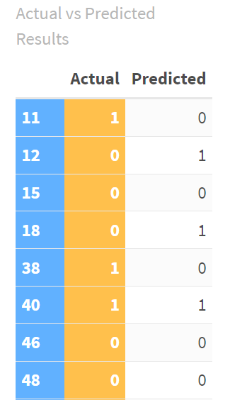
Let's now illustrate the results of the Logistic Regression model we trained to predict how it works against the test dataset. In this code snippet, we first validate the symmetry between the training and test datasets, create a predictions data frame (including the actuals and predictions), and classify the predictions into a binary classification. We then create a table to present the results.

data_test_df <- data_test_df[, names(data_train_df)]

predictions <- predict(model, newdata = data_test_df, type = "response")
predicted_classes <- ifelse(predictions > 0.5, 1, 0)

result_summary <- data.frame(
  Actual = data_test_df$WIN,
  Predicted = predicted_classes
)

kable(result_summary, format = "html", caption = "Actual vs Predicted Results") %>%
  kable_styling(bootstrap_options = c("striped", "hover", "condensed", "responsive"), full_width = F) %>%
  column_spec(1, bold = TRUE, color = "white", background = "dodgerblue") %>%
  column_spec(2, bold = TRUE, color = "white", background = "orange")

Below is an excerpt from the broader table, so you can see the actual result (win, 1, or loss, 0) versus the prediction from the logistic regression model.

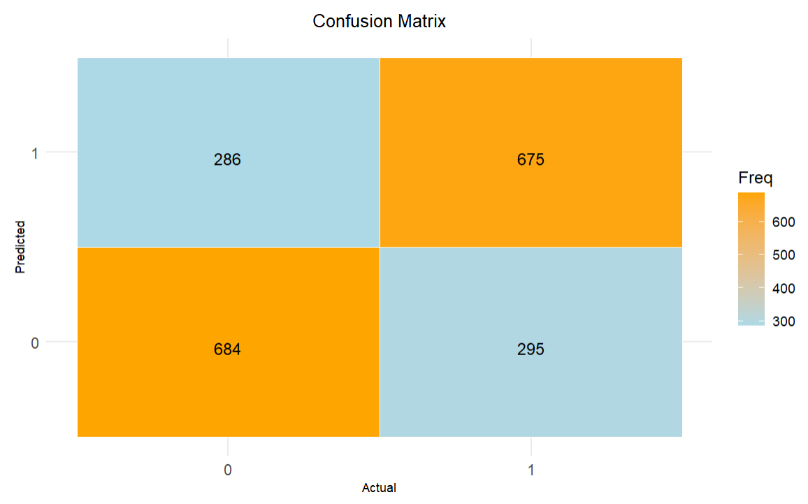
The next step is to create a confusion matrix, which summarizes the actual results and predictions into a matrix where you can see how well the model performed. This next code snippet creates the confusion matrix, converts it into a data frame and then visualizes the results.

conf_matrix <- table(Predicted = predicted_classes, Actual = data_test_df$WIN)

conf_matrix_df <- as.data.frame(as.table(conf_matrix))

ggplot(data = conf_matrix_df, aes(x = Actual, y = Predicted, fill = Freq)) +
  geom_tile(color = "white") +
  geom_text(aes(label = Freq), vjust = 1) +
  scale_fill_gradient(low = "lightblue", high = "orange") +
  labs(title = "Confusion Matrix", x = "Actual", y = "Predicted") +
  theme_minimal() +
  theme(
    plot.title = element_text(hjust = 0.5, size = 20),
    axis.title.x = element_text(size = 15),
    axis.title.y = element_text(size = 15),
    axis.text = element_text(size = 12)
  )
  

Below are the results of the model using the confusion matrix. The way to read the matrix is how well the model predicted the results. This model appears pretty decent with the following results shown in the matrix.

• True Positives (TP): 675 (Predicted 1, Actual 1)
• True Negatives (TN): 684 (Predicted 0, Actual 0)
• False Positives (FP): 295 (Predicted 1, Actual 0)
• False Negatives (FN): 286 (Predicted 0, Actual 1)

Our next step is to measure the model through different metrics, such as accuracy, sensitivity, specificity, positive predictive value, and so on. The code snippet below creates a data frame and view from the model results across a set of available metrics.

performance_metrics <- data.frame(
  Metric = c("Accuracy", "Sensitivity", "Specificity", "Pos Pred Value", "Neg Pred Value", "Kappa", "Balanced Accuracy"),
  Value = c(
    confusion_matrix$overall["Accuracy"],
    confusion_matrix$byClass["Sensitivity"],
    confusion_matrix$byClass["Specificity"],
    confusion_matrix$byClass["Pos Pred Value"],
    confusion_matrix$byClass["Neg Pred Value"],
    confusion_matrix$overall["Kappa"],
    confusion_matrix$byClass["Balanced Accuracy"]
  )
)

kable(performance_metrics, format = "html", caption = "Performance Metrics") %>%
  kable_styling(bootstrap_options = c("striped", "hover", "condensed", "responsive"), full_width = F) %>%
  column_spec(1, bold = TRUE, color = "white", background = "dodgerblue") %>%
  column_spec(2, bold = TRUE, color = "white", background = "orange")

The results of the model are as follows:

• Accuracy is 70%. The model is right 70% of the time.
• Sensitivity is 70%. The model correctly identifies 70% of the actual losses.
• Specificity is 70%. The model correctly identifies 70% of the actual wins.
• Precision for Losses is 70%. When the model predicts a loss, it is right 70% of the time.
• Precision for Wins is 70%. When the model predicts a win, it is right 70% of the time.

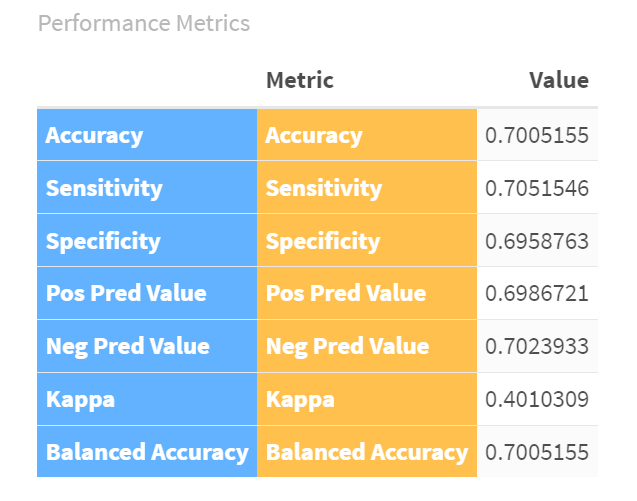
In sum, the Logistic Regression model is fairly accurate, correctly predicting the outcome of games 70% of the time. It has balanced performance in identifying both wins and losses. This means the model is a good starting point, but there's room for improvement to make it even more accurate.

Plotting an ROC Curve to Visualize the Logistic Regression Model

The last step is to visualize the model using an ROC curve. The ROC (Receiver Operating Characteristic) curve is a graphical representation used to evaluate the performance of a classification model. It helps us understand how well our model can distinguish between different classes (wins vs. losses) and provides a single metric (AUC) to summarize its performance.

The code snippet below creates the ROC curve using the predictions and then plots the True Positive Rate (TPR) and False Positive Rate (FPR). The TPR, also known as sensitivity or recall, is plotted on the y-axis and represents the proportion of actual wins that were correctly predicted. The FPR represents the proportion of actual losses that were incorrectly predicted as wins by the model.

roc_curve <- roc(data_test_df$WIN, predictions)
auc_value <- auc(roc_curve)

roc_plot <- ggroc(roc_curve, color = "blue", size = 1.2) +
  geom_abline(linetype = "dashed", color = "red") +
  labs(title = "ROC Curve", 
       subtitle = paste("AUC =", round(auc_value, 2)),
       x = "False Positive Rate", 
       y = "True Positive Rate") +
  theme_minimal() +
  theme(
    plot.title = element_text(hjust = 0.5, size = 20, face = "bold"),
    plot.subtitle = element_text(hjust = 0.5, size = 15),
    axis.title.x = element_text(size = 15),
    axis.title.y = element_text(size = 15),
    axis.text = element_text(size = 12),
    panel.grid.major = element_line(color = "gray90"),
    panel.grid.minor = element_line(color = "gray95")
  ) +
  annotate("text", x = 0.7, y = 0.2, label = paste("AUC =", round(auc_value, 2)), color = "blue", size = 5, hjust = 0)

print(roc_plot)

The ROC curve of our Logistic Regression model is plotted in blue. The curve is well above the diagonal line, indicating that our model performs better than random guessing. Further, the AUC value is displayed on the plot. In our example, it is approximately 0.75, suggesting that our model has good discriminatory ability.

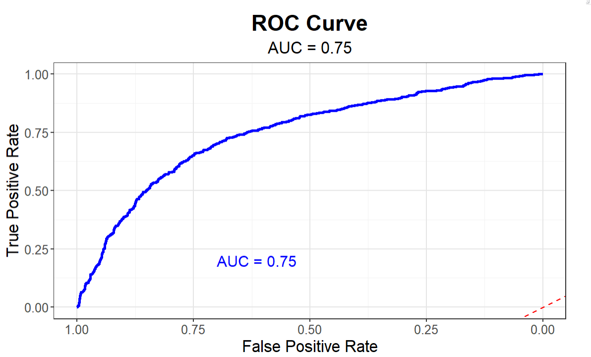
In summary, our model is a relatively performant model having a predictive power of about 70%, meaning when applied as is, it will predict the outcome of a game as a win or loss about 70% of the time.

Could you improve the predictive strength of this model? Sure. You could reduce the input variables that don't contribute to helping; you could test and add other input variables; and you could tweak the weightings or context of statistics, such that you either create and/or include variables that are closer to the goal-scoring events (e.g., shots for within a certain distance to the net).

We'd encourage you to take the R code and swap out different input variables from the dataset (or ones you customize) to improve the model to, say, 80%.

Check out our quick-hit video on YouTube:

Summary

In this newsletter, we introduced you to the Logistic Regression algorithm, a binary classification model that has many general applications and practical applications for hockey. We then demonstrated how to implement the Logistic Regression model by creating a logistic model to predict wins. In our model, we used five calculated hockey statistics, which are listed below.

• Shots For Percentage (SF_PCT)
• Expected Goals For Percentage (XGF_PCT)
• Corsi For Percentage (CF_PCT)
• Fenwick For Percentage (FF_PCT)
• High Danger Goals For Percentage (HDGF_PCT)

We found that using these inputs into the Logistic Regression model, our model predicts with 70% accuracy – which is a pretty decent outcome. We also found that not all calculated metrics contributed to the model, for example FF_PCT didn't help the model.

You can explore building your own Logistic Regression model using the same or a different set of hockey statistics with the goal of improving on the 70% level of the current model. The dataset and code for the walkthrough are below.

• Multi-season Team Statistics Dataset
• R Code - Logistic Regression Analysis to Predict Wins

We've also included some additional references in case you want to explore more readings on Logistic Regression models.

• Analysis of Factors Contributing to Hockey Wins
• Logistic & Linear Regression in Hockey
• What Wins Hockey Games?
• Estimating Player Contribution in Hockey with Regularized Logistic Regression

Subscribe to our newsletter to get the latest and greatest content on all things hockey analytics!