Predicting the Stanley Cup Playoffs: Finding the Perfect Model

At a Glance
- Three Predictive Techniques
- Goals For per Game (GFPG)
- Pythagorean Win Percentage (PWP)
- Bayesian Probability
- Which Method Should You Use?
Three Predictive Techniques
Every year, NHL fans, analysts, and sportsbooks attempt to forecast who will hoist the Stanley Cup. However, the playoffs are a reset moment; the top teams are now contending for the coveted Cup and the game, pace, and aggression are all elevated. At the same time, the refs tend to let calls slide, so the game is different. So, predicting the winner is a blend of art, science and a generous dose of luck.
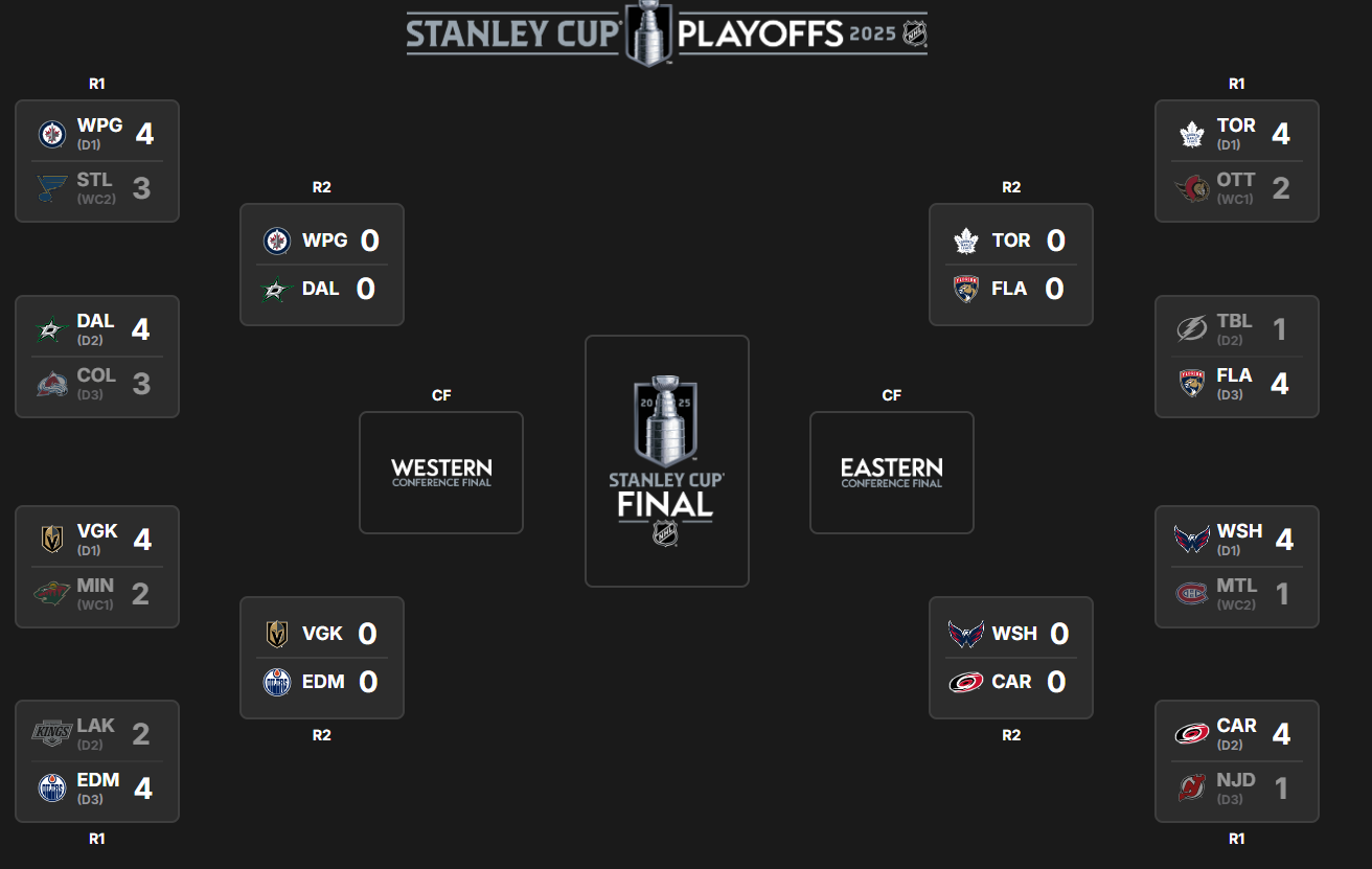
As of this writing, Round 1 is complete and the Western Conference was tighter and more competitive than the Eastern Conference. These games have been fun to watch with surprises all over the ice. Case in point: the Dallas comeback in the heels of Drury's penalty and Winnipeg tying it up with 1.6 seconds to go and then taking it in double overtime. Just wow! And Round 2 is shaping up to be a seriously competitive round. So, amidst the chaos how do you predict a winner?
The short answer is there's no perfect way, but in this article we'll explore three ways to predict the Stanley Cup champion:
- Goals For per Game (GFPG)
- Pythagorean Win Probability (PWP)
- Bayesian Probability
Each method offers a different lens on forecasting, from raw scoring power to deeper probabilistic reasoning coupled with more dynamic predictions.
Feeling lazy? Check out the quick-hit video below.
Goals For per Game (GFPG)
Goals For per Game (GFPG) is a decent, simple starting point (especially if you're new to predictive modeling) because teams that score the most win the most. If you're new to predicting wins, this is one of the easier techniques to learn and apply.
Implementing the GFPG Model
You implement the GFPG model by first gathering each playoff team's average GFPG from the regular season and ranking the teams by GFPG. For example, here are the 2024-2025 playoff teams with their average GFPG for the season, sorted highest to lowest. This is the first input into your model.

You use the GFPG stats to create a probability proportional to the GFPG for each team. You can do this in different ways, but using a ratio is one of more straightforward ways, such as:
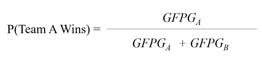
With the GFPG and a probability, you create the matchups and compare which team is higher. Those teams that are higher would be the predicted winner.
If we take this year's playoffs and run the numbers, here is the forecast you get from the GFPG model. This model shows the matchup for Round 1, the respective team's GFPG and WP (listed in order as they appear in the first column) and then the predicted winner based on which team has the greater value.
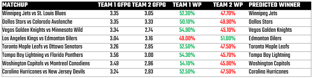
With Round 1 behind us, the accuracy of these predictions was 87.5%.
Testing
You can test the model by backtesting, which is where you take historical data and run your model against that data to test the efficacy of your model. That is, compare historical playoff results to regular-season GFPG and test how far the highest GFPG team advances each year.
Pros and Cons
The pros of the GFPG model is it's easy to calculate and you don't need a lot of coding skills to do it. By downloading the data from Hockey Reference (or another hockey data provider) and arming yourself with a simple spreadsheet, you can replicate what we've created above.
However, the cons are it ignores other aspects of the game, such as defensive ability and goaltending strength. It also assumes offense alone is equally effective in playoff environments. For example, hockey is much more physical in the playoffs, teams score 0.20 less goals on average in the playoffs and teams that go the distance often have standout goaltending. And the "hot goalie factor" can completely erase a GFPG advantage.
At the end of the day, GFPG is more of a "blunt predictive object" and can be used for initial point-in-time directionality, but you need additional context for precision.
Pythagorean Win Percentage (PWP)
Inspired by Bill James in baseball, Pythagorean Win Percentage (PWP) – sometimes referred to as Winning Percentage – translates goal differential into a projected winning percentage. It is a model that adjusts for both offense (goals scored) and defense (goals conceded). The PWP calculation incorporates three factors:
- Goals For (or GFPG)
- Goals Against (or GAPG)
- Sport-Specific Exponent (which is between 2 to 2.2 for hockey)
The formula for PWP is as follows:
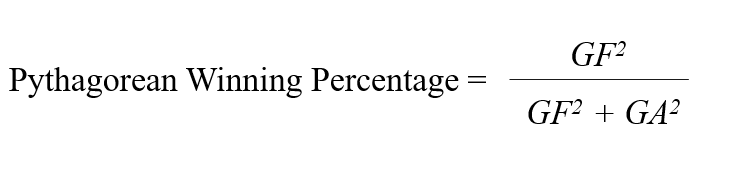
In the formula, GF is Goals For, GA is Goals Against, and the exponent is a factor that is specific to hockey.
Implementing the PWP Model
You calculate the PWP for every playoff team based on their regular season numbers. And then you use this as a baseline for that team's "true strength" rating. You can calculate it on a game-by-game basis and then take the average or take the season totals and calculate it that way. You can then predict each playoff matchup using the PWP estimates. For example, below is a snapshot of the total GF and GA for each team in the 2024-2025 Regular Season. We then use the following Excel formula to calculate the PWP column:
=([@[2024-2025 GF]]^2)/([@[2024-2025 GF]]^2+[@[2024-2025 GA]]^2)
We then ranked the table using the PWP and highlighted that column using conditional formatting. The below was the result.
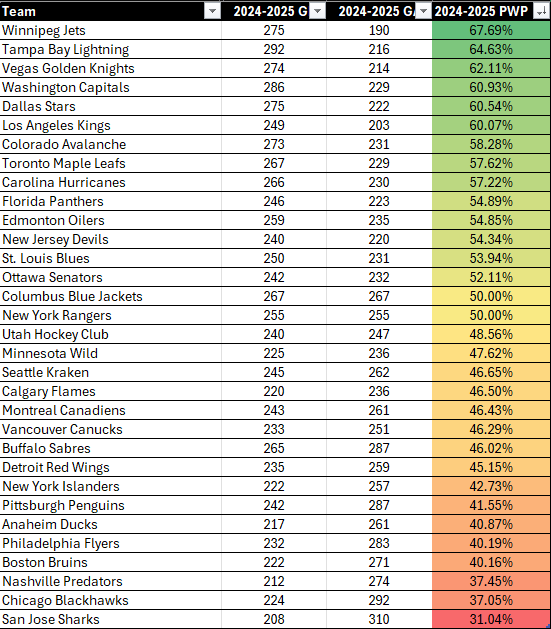
To interpret these results, take Winnipeg and Chicago. Separately, the PWP translates into the following:
- Winnipeg’s PWP of .677 means based on their goals for and against, Winnipeg played like a team that should win 67.7% of their games.
- Chicago’s PWP of 0.371 means they performed like a team that should win only 37.1% of their games.
Thus, the PWP column gives you an indicator of how well a team could do (in isolation). If you want to compare two teams, then you'd want to calculate a Win Probability using the PWP for each team. For example, if we wanted to calculate the Win Probability for Winnipeg, we could use the following formula:
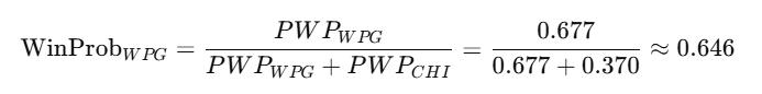
The result of this calculation is that Winnipeg would have about a 64.6% chance to beat Chicago in any given game using the PWP-based modeling.
Simulating Round 1 using PWP
If we run the above PWP results through a one-time simulation of the Round 1 teams, you get the following results. The Matchup column shows who's playing who, the Team 1 PWP is the PWP for the team that is listed first (e.g., Winnipeg) and the Team 2 PWP is the PWP for the team that is listed second (e.g., St. Louis). The Predicted Winner is the prediction of which team would be forecasted to win.
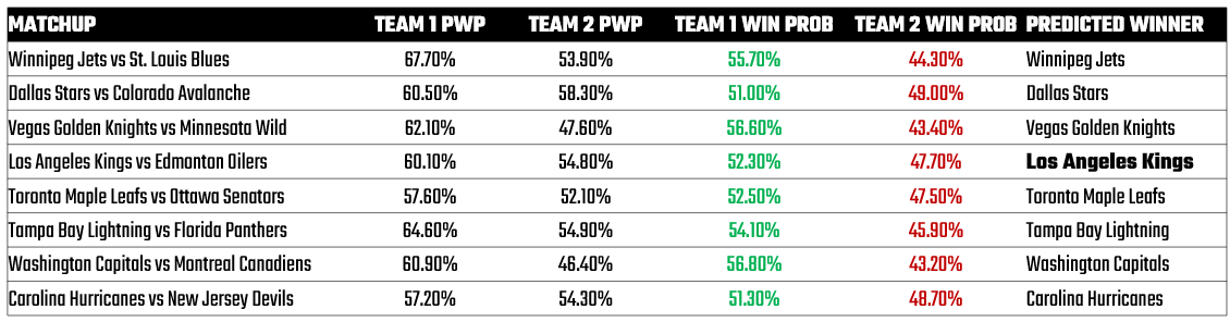
Note that the outcomes that are predicted by the PWP are similar to those resulting from the GFPG model. The only difference is the PWP predicts LA winning instead of Edmonton.
With Round 1 behind us, the accuracy of these predictions was 75%.
Testing the Method
You can also backtest the PWP model – similar to what you would do with the GFPG model. Specifically, you collect the previous year's regular season data, calculate the PWP for each team and model out the brackets for those playoffs (that have already happened) using a converted Win Probability. You'd then take the results of the matchups and compare the predicted PWP-based standings to actual playoff performance. You can then calculate an accuracy rate based on the number of correct results out of the total matchups.
Pros and Cons
The pros are that it balances offense and defense and doesn't just focus on offensive production through goal-scoring. It also smooths out luck or lopsided scores and upsets. And while similar in outcomes in this newsletter, PWP is generally a better predictor than raw standings or the GFPG.
The cons, however, are that the PWP model still assumes regular season metrics transfer cleanly to playoffs. We know that playoff hockey is different – for all the reasons we stated earlier. In short, while both the GFPG and PWP models are based off historical performance (by using regular season metrics), you'd need to create a model that updates after each game to improve the performance of the model.
Also, the PWP model doesn't capture goalie performance streaks or special teams nuances given the limited variables within the model. And the PWP model loses sensitivity to teams with extreme goal differentials, which may be skewed by blowouts.
That said, we believe that the PWP model is a strong baseline. It's simple, effective, and theoretically broader than relying on only Goals For.
Bayesian Probability Updates
As we've seen, the GFPG and PWP models are based on regular season statistics that are applied to future playoff performance. Implemented as a point-in-time model, this has the drawback of not considering what's happening as games progress within the playoffs. Bayesian probability allows you to update calculations about a team's predictive strength as new information comes in, such as the results of a game. You can also capture broader statistical dimensions within your model.
Implementing Bayesian Probability
You implement a Bayesian Probability model by starting with a prior probability. This is your belief (or hypothesis) about an event before observing any new data. For example, there’s a 60% chance the home team will win before seeing the lineup. Using a likelihood factor based on evidence, a Bayesian Probability model is updated through a posterior probability. After each game, you update the team's posterior probability of winning the series based on different factors, such as:
- Game result (win or loss)
- Shots For vs Shots Against
- Expected Goals (xG) differential
Let's walk through an example: Will Colorado win Game 7?
The first step is to set the prior probability. Let's assume we use PWP to generate this number and the result is a prior probability of 60% that Colorado will win Game 7. Statistically, this is written out as P(Win) = .60.
We now need to factor in any new evidence we have that will allow us to re-calculate the probability. So, let's factor in the fact that Colorado didn't have home-ice advantage in Game 7. And based on our calculations, the probability that Colorado wins on the road is 46%.
With the prior probability and the 46% chance of winning on the road, we can use probabilistic statistics to calculate a final posterior probability. And after you do this, the posterior probability is 51.5% – calculated at the game level. You can also use evidence within a game to update the Bayesian Probability during a game. For example, with the Drury penalty in the third period, home-ice advantage and Rantanen having a stand-out game, the edge within Colorado's posterior probability was diminished.
Testing the Method
To test the Bayesian Probability method, you can run Bayesian updates after each playoff game historically. After you've done this, you compare the updated series probabilities to actual outcomes.
Pros and Cons
The pros of the Bayesian Probability method are that the model adapts as the series unfolds; it's not stuck to pre-series assumptions (e.g., calculating the probabilities solely using the regular season statistics). The model also reflects momentum, injuries, goalie changes, and style shifts – so it captures more dimensionality. And finally, it can be automated to dynamically adjust predictions after every game.
The cons are that it's more complex and requires more technical sophistication (Bayes theorem implementation) and an understanding of how statistical probability works. Also, the risk of overreacting to small sample sizes (one fluke game can heavily sway model). And lastly, it's harder to explain to casual audiences – no less for them to put into practice.
The bottom line is that Bayesian Probability models are the gold standard if you can build them well. They capture playoff chaos and momentum better than static season-long models. They can also operate at different levels of event granularity – e.g., at the game level, period level or even shift level.
If you're looking for a great application of Bayesian Probability, check out NHL Forecasts, which updates the probabilities regularly based on different evidence.
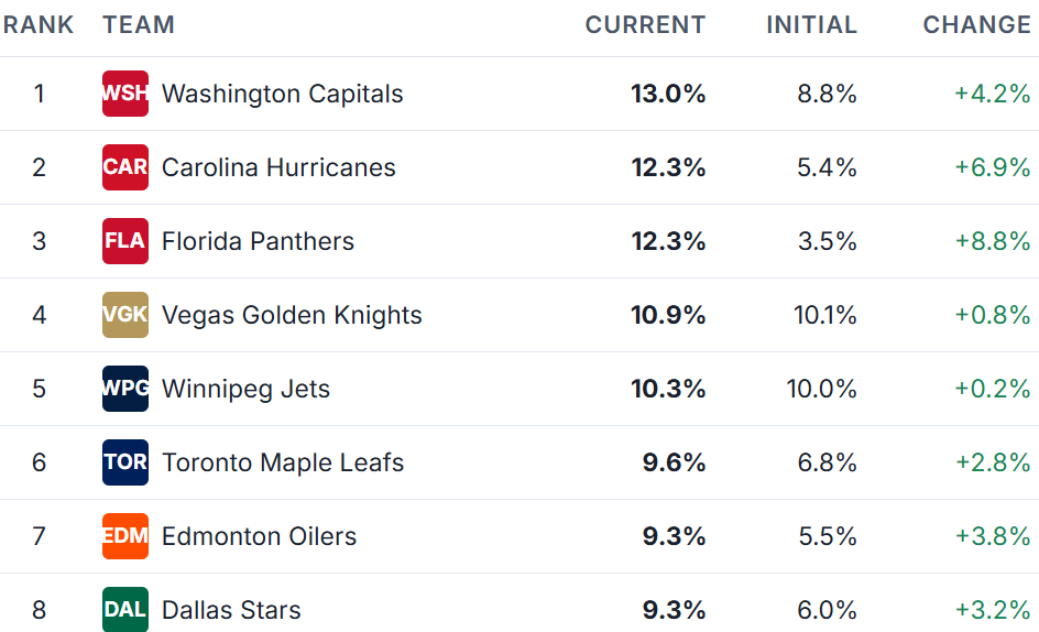
The site describes its methodology, so you can get a sense for how complex the "evidence" can be when calculating the posterior probability.
Summary
In this edition, we walked through three different ways to predict the NHL Stanley Cup playoffs:
- GFPG - which uses the regular seasons Goals For per Game (GFPG) to calculate Win Probabilities for each team.
- PWP – which uses Goals For, Goals Against (taken from the regular season) and a sport-specific exponent to calculate Win Probabilities for each team.
- Bayesian Probability - which uses the results of each game to adjust the Win Probability, such that the forecast is more dynamic and current to the games being played.
The table below shows where each method might be appropriate to use.
| Method | Best Use Case |
|---|---|
| GFPG | Quick, surface-level power ranking |
| PWP | Strong season-wide predictive model |
| Bayesian Probability | Best real-time playoff series predictor |
Our advice would be to start small with the GFPG and PWP methods and understand the process of building the Win Probabilities and then applying them across a series. And then work into the more complicated Bayesian Probability.
In the end, no model captures the full magic and madness of the Stanley Cup playoffs — but using smart, evolving data methods gets you far closer than gut instinct alone.
Subscribe to our newsletter to get the latest and greatest content on all things Data, AI and Hockey!
Member discussion