Preparing for the NHL 2024 Draft: Top 50 Prospect Analysis

In this Edition

• Draft 2024 Prospect Newsletter Series Recap
• About the Top 50 Prospects Dataset
• Top 50 Draft Prospects Exploratory Data Analysis
• Top 50 Draft Prospects Dashboard

Draft 2024 Prospect Newsletter Series Recap

This is Week 5 in our six-week newsletter series on Preparing for the NHL Draft 2024. In the first four editions, we covered the following topics:

• Week 1 Edition: Introduction to the six-week series.
• Week 2 Edition: Overview of the data discovery process using Microsoft Excel and a high-level walkthrough using the team stats dataset.
• Week 3 Edition: Analyzing the NHL teams for strengths and weaknesses across offense, defense and goaltending.
• Week 4 Edition: Analyzing the NHL 2024 Draft prospects including a high-level analysis, data discovery using Excel and a Power BI dashboard including 477 incoming prospects.

In this week's edition, we'll more deeply explore the NHL 2024 Draft prospects focusing on the top 50 prospects through an Exploratory Data Analysis (EDA) and a Power BI dashboard.

About the Top 50 Prospects Dataset

To start, the top 50 prospects dataset can be downloaded from here. After you download the data, you'll see data similar to the below screenshots.

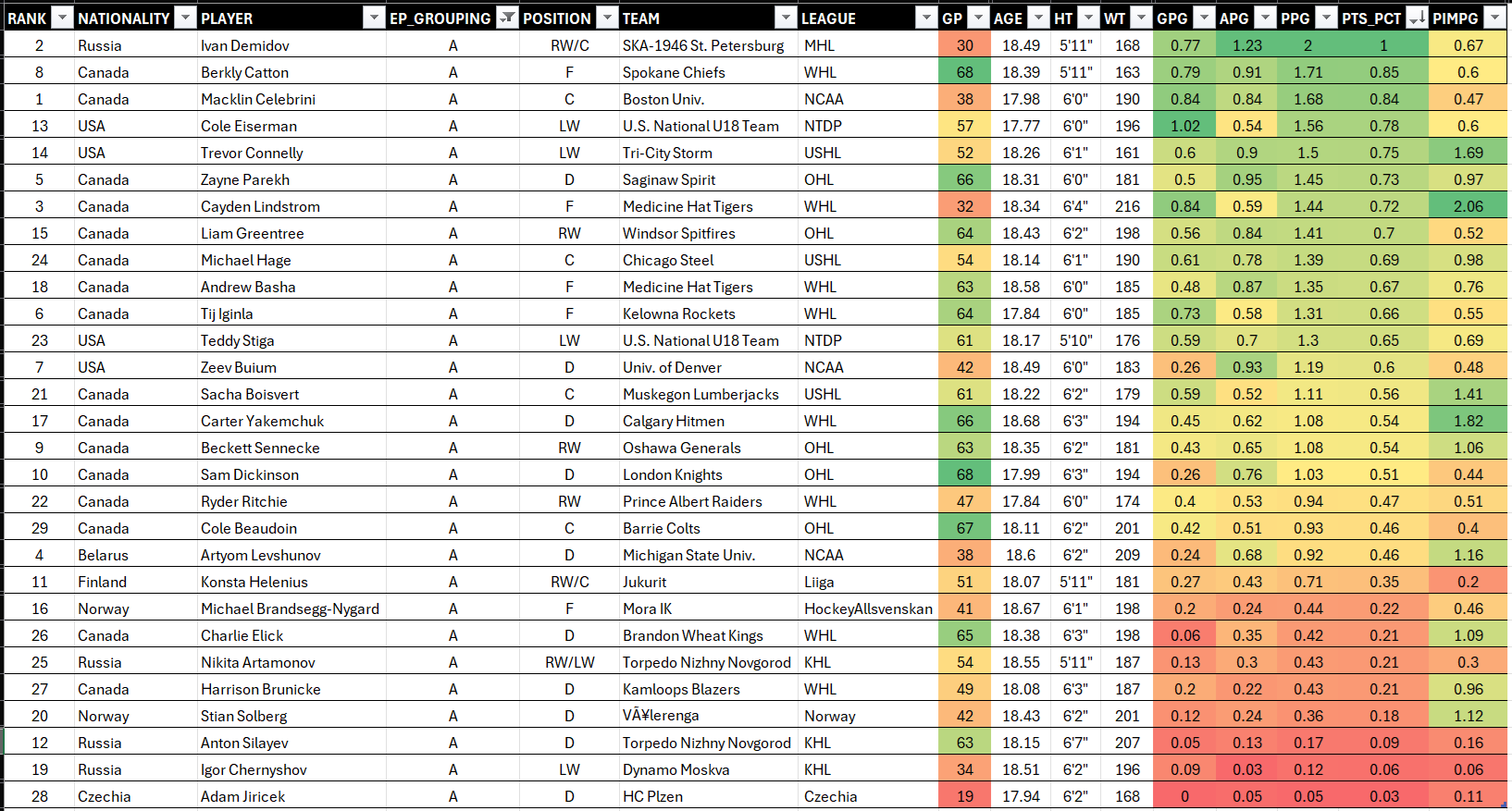
The dataset is broken into prospect metadata, which includes RANK, NATIONALITY, PLAYER, EP_GROUPING (Elite Prospect's draft round recommendation), POSITION, TEAM, and LEAGUE. You can see example metadata from the dataset below.

The rest of the data is raw and calculated statistics (e.g., GP, G, A, PTS_PCT, etc.) or prospect properties such as AGE, HT (height), WT (weight), and S (shoots). You can see example data from the dataset below.

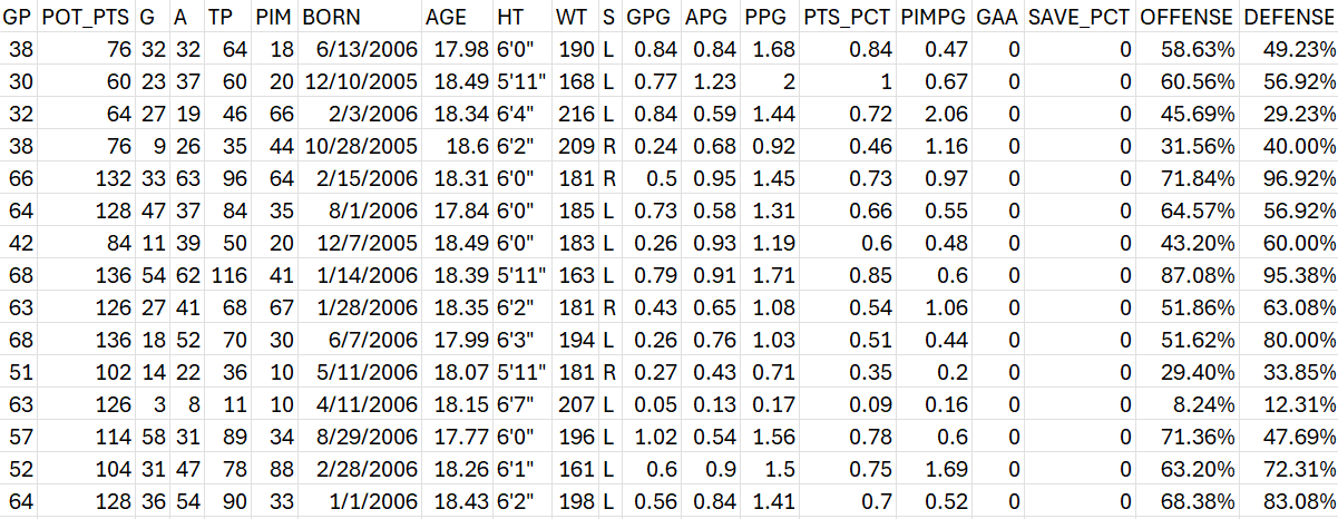
We'll use this dataset to create the EDA and the Top 50 Prospects Dashboard.

Top 50 Draft Prospects Exploratory Data Analysis

The EDA is composed of three parts:

1. We'll first explore the summary statistics for the top 50 prospects
2. Then we'll compare Group A and B prospects
3. And finally, we'll cluster the top prospects in Group A (based on one statistic)

You should then be able to extend the above to your liking – e.g., exploring specific statistics, creating your own composite metrics, choosing different clustering criteria, and so on.

Summary Statistics

Let's first look at the summary statistics for the top 50 prospect dataset, which provide a good overview of the dataset.

Here are some key observations:

• Games Played (GP): Ranges from 14 to 68 with an average of about 53 games.
• Goals (G): Ranges from 0 to 58 with an average of about 21 goals.
• Assists (A): Ranges from 1 to 63 with an average of about 31 assists.
• Total Points (TP): Ranges from 1 to 116 with an average of about 52 points.
• Penalty Minutes (PIM): Ranges from 0 to 120 with an average of about 39 penalty minutes.
• Weight (WT): Ranges from 148 to 216 pounds with an average weight of about 186 pounds.
• Goals Per Game (GPG): Ranges from 0 to 1.02 with an average of about 0.39 goals per game.
• Assists Per Game (APG): Ranges from 0.03 to 1.23 with an average of about 0.56 assists per game.
• Points Per Game (PPG): Ranges from 0.05 to 2.00 with an average of about 0.95 points per game.
• Points Percentage (PTS_PCT): Ranges from 0.03 to 1.00 with an average of about 0.47.
• Penalty Minutes Per Game (PIMPG): Ranges from 0 to 2.06 with an average of about 0.71.

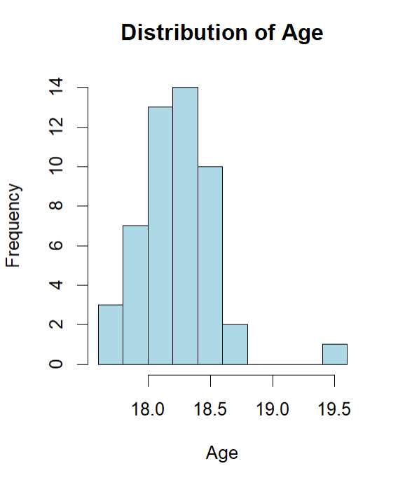
Our next stop is age, which generally falls into a normal distribution, ranging from 17.75 to 19.44 years with an average age of about 18.26 years. The one outlier is Jesse Pulkkinen from Finland who is 19.44 years of age.

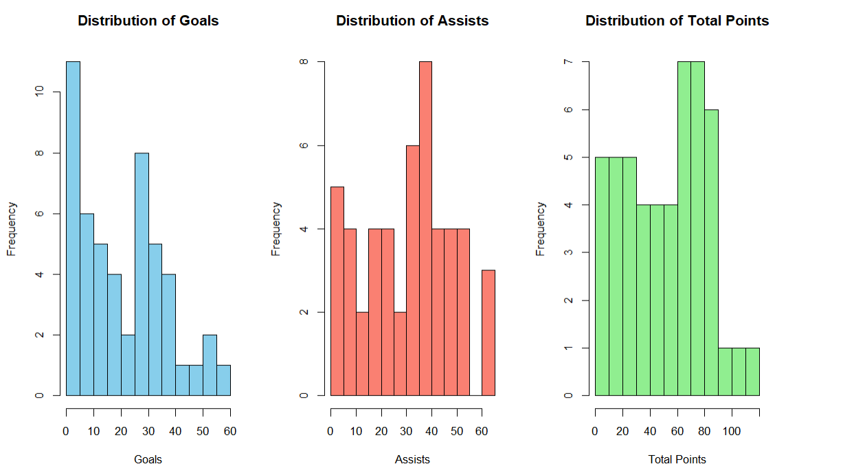
When we look at goals, assists and total points in more detail, you see some interesting trends among the top 50 prospects. For example, there's a sizeable goal-scoring cohort that have scored 30 or more goals and an equal if not bigger cohort for assists. Though, very few (n = 3) have achieved more than 90 total points – Berkly Catton, Terik Parascak and Zayne Parekh (all hailing from Canada).

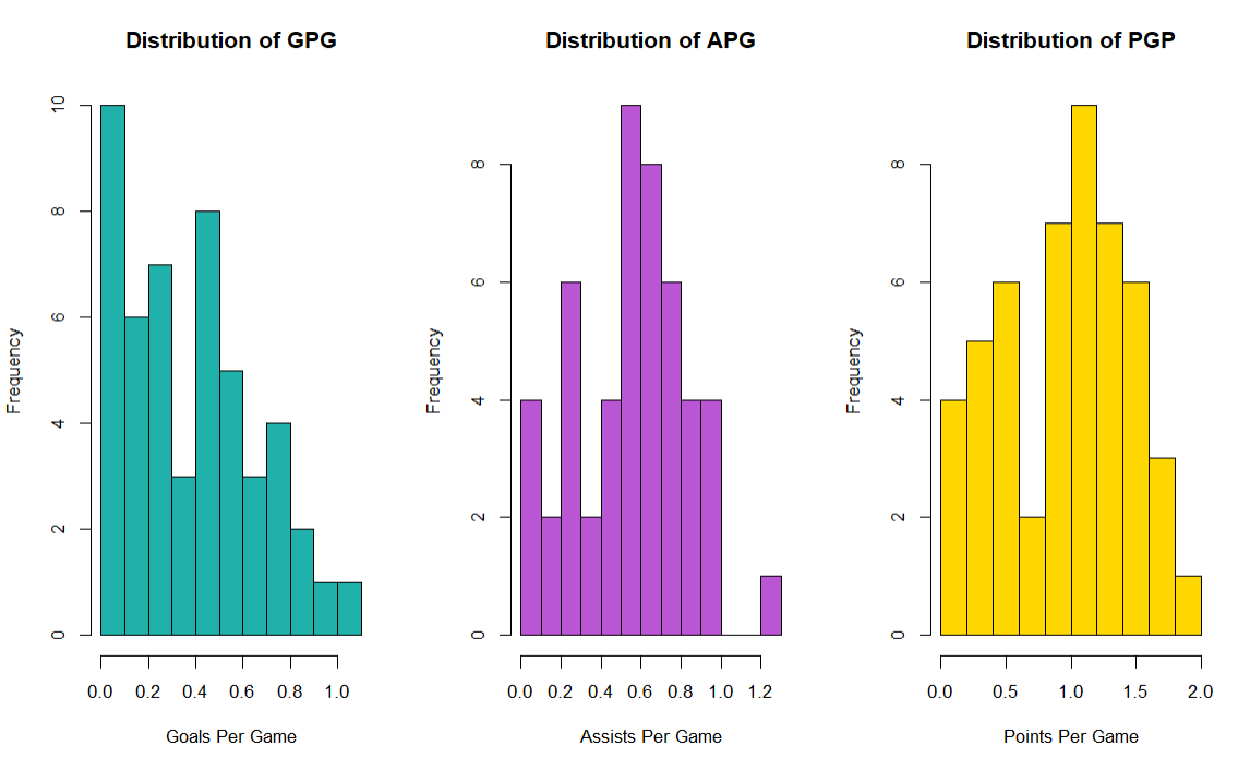
When you look at production through the "per game" lens, you see a right skew for goals per game (GPG), a more normalized assists per game (APG) and a somewhat normalized points per game (PGP). The outliers here are:

• Cole Eiserman and Dean Letourneau for GPG (from USA and Canada respectively);
• Ivan Demidov for APG (from Russia); and
• Ivan Demidov, Dean Letourneau, Berkly Catton, and Macklin Celebrini for PGP (Demidov from Russia and the rest from Canada).

Let's now explore Elite Prospects' Group A and Group B within the top 50 prospects.

Compare Group A and Group B

Elite Prospects has a grading system that classifies draft prospects into five groups, A through F. In our Top 50 dataset, you'll find all those in Group A with some prospects in the top 50 in Group B.

Let's start by adding some conditional formatting to the dataset, so you can compare the prospects across the available statistics. To do this:

1. Open the Top 50 Prospect dataset in Microsoft Excel.
2. Click on the A1 cell, and select Format as Table, select the table style, range and click OK.
3. Select the columns you want to format and select Conditional Formatting, Color Scales and choose a specific color scale.

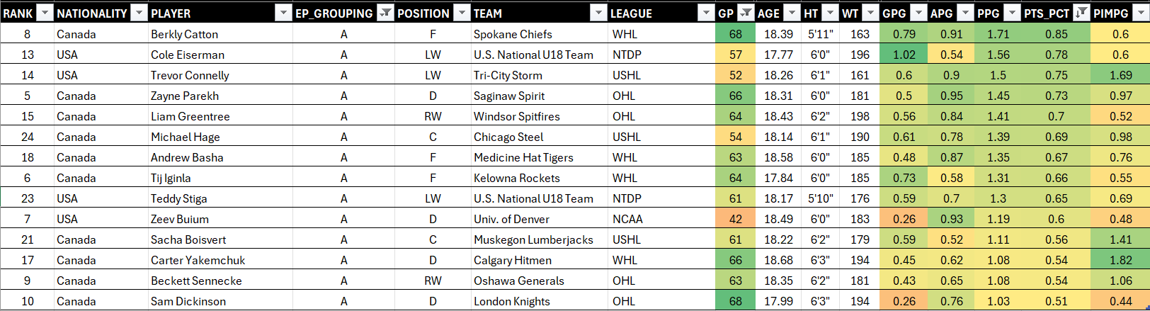
You'll then have a heatmap for your Top 50 list across the different statistics, which you can then explore through sorting, filtering, etc. For example, below is a heatmap of Group A prospects, ranked by PTS_PCT. You should see something similar to the below, which you can use to visually compare where different prospects may be stronger or weaker than one another.

For example, the RANK column uses the ranking from the Elite Prospect NHL 2024 Guide, so it's interesting to see that while some of the top ten prospects hold, some lower-ranked prospects find their way into the top ten – for example, Cole Eiserman, Trevor Connelly, Liam Greentree, Michael Hage, and Andrew Basha.

We wanted to filter the Group A data view more, so we filtered for greater than 40 games (our arbitrary representation of experience) and filtered for PTS_PCT greater than 0.5. This narrowed the list down to 14 players, and at the top was Berkly Catton.

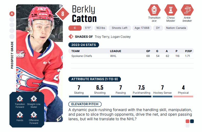
We've included the summary for Catton below, which gives you a high-level summary and assessment and also gives additional information around his ratings and scouting commentary. Here you can see the EP ratings are broader and more qualified through scouting reports. For example, according to EP's assessment of Catton, "there’s always a catch with any prospect, and this is true of Catton. In his case, it’s one of efficiency. He’s prone to throwing pucks away with hope passes and lacks that extra layer of patience that defines most top playmakers. One can wonder to what extent playing on a team with as little firepower as Spokane helped foster these bad habits, but they’re there all the same."

Let's turn to Group B to explore those prospects in the top 50 ranking. When you filter on Group B (EP_GROUPING), you should see something similar to the below. We've also sorted here again on PTS_PCT, so you get a sense for who has the greater point production across the players.

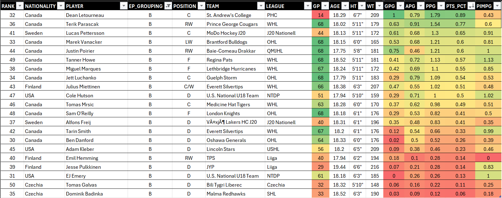
If we apply the same filters as we did to Group A (GP greater than 40 and PTS_PCT > 0.5), the list thins out a bit. Comparatively speaking, the Height and Weight of these players are smaller than the top Group A prospects. Further, the Points Percentage is lower as well. This makes some sense as you'd expect the stand-out players to be in Group A.

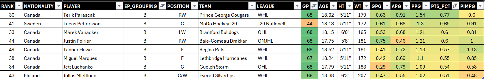
Nonetheless, let's include the EP summary on Terik Parascak, who tops our Group B list and ranking by the analytics.

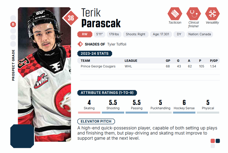
According to the EP report, "[i]t would be very wrong to assume that Parascak was merely a conduit for the plays of his older linemates. He showed plenty of NHL skills in his breakout season and likely has the capacity to become more of a driver in time."

At this point, you should be able to continue to explore the Top 50 Prospects dataset (creating more of your own analyses) and use the Elite Prospect 2024 Draft Guide to get more detailed information about your prospects of interest.

So, for the final part of our analysis, we'll conduct a K-Means Cluster analysis; that is, a way to cluster players around specific statistics.

K-Means Cluster Analysis

Our goal with the cluster analysis is to group the top prospects using a specific statistic. For this analysis, we'll use some R code to create a K-Means cluster analysis based on Points Percentage (PTS_PCT).

There are three steps to the Cluster analysis:

1. Load and filter the data for Group A.
2. Determine the optimal number of groups (or clusters) in the dataset.
3. Create and plot the K-Means clusters.

The below code snippet is R code built using RStudio. It reads in the CSV file, uses the dplyr library to create a filtered data frame, scales the data, and then calculates the sum of squared errors (SSEs) and plots them.

library(dplyr)
library(ggplot2)
library(factoextra)

data <- read.csv("Top_50_Prospects.csv")

group_a <- data %>% 
  filter(EP_GROUPING == "A")

group_a_scaled <- scale(group_a$PTS_PCT)

sse <- sapply(1:10, function(k) {
  kmeans(group_a_scaled, centers = k, nstart = 25)$tot.withinss
})

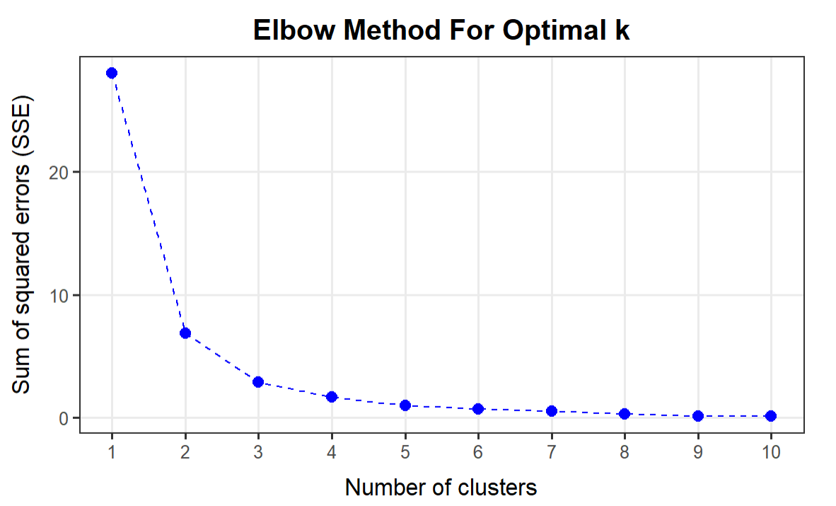
plot(1:10, sse, type = "b", pch = 19, frame = FALSE, 
     xlab = "Number of clusters", ylab = "Sum of squared errors (SSE)",
     main = "Elbow Method For Optimal k")

The optimal number of clusters you would configure for your K-Means analysis typically lies at the "elbow" of this plot. So, in the plot below the bend occurs at 3.

In the next dataset, we set the number of clusters (optimal_k) to 3 and then create and plot the cluster.

set.seed(42)
optimal_k <- 3  
kmeans_result <- kmeans(group_a_scaled, centers = optimal_k, nstart = 25)

group_a$Cluster <- kmeans_result$cluster

ggplot(group_a, aes(x = PLAYER, y = PTS_PCT, color = factor(Cluster))) +
  geom_point(size = 3) +
  theme_bw(base_size = 10) +
  geom_hline(yintercept = 0.62, linetype = "dashed", color = "red", size = .5) +
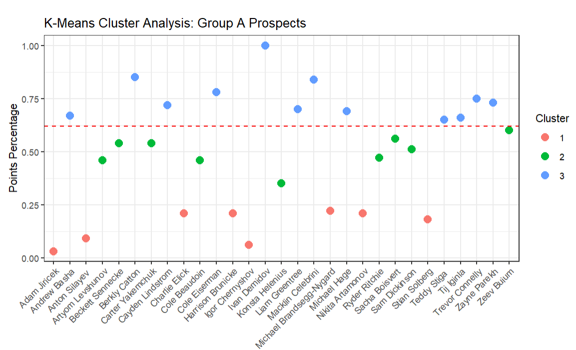
  labs(title = "K-Means Cluster Analysis: Group A Prospects",
       x = "Players", y = "Points Percentage", color = "Cluster") +
  theme(axis.text.x = element_text(angle = 45, size = 8, hjust = 1))

The resulting plot (using Points Percentage) with the help of a dotted red line shows the cluster of prospects who are highest on the list. In the plot below, these are the blue dots that are highest on the plot, separated from the green and red dots by the red dotted line.

Broken out, here are the top 12 prospects in Group A from the K-Means cluster analysis, along with their corresponding Points Percentage (PTS_PCT) score. In this final view, we've ranked the prospects by largest to smallest PTS_PCT.

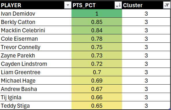
We've only looked at point production, so you should explore the dataset across other positions and statistics, so you both get to a comfortable ranking for yourself – across forwards and defense – and also evaluate the prospects in different ways.

Top 50 NHL Draft Prospect Dashboard

In our Week 4 newsletter, we created a first version of the NHL Draft 2024 Prospect dashboard. However, we included all of the listed prospects in the Elite Prospects Draft Center. This week, we'll only cover the top 50 prospects.

For the Top 50 Prospect Analysis cover page, we updated the text and re-used the design.

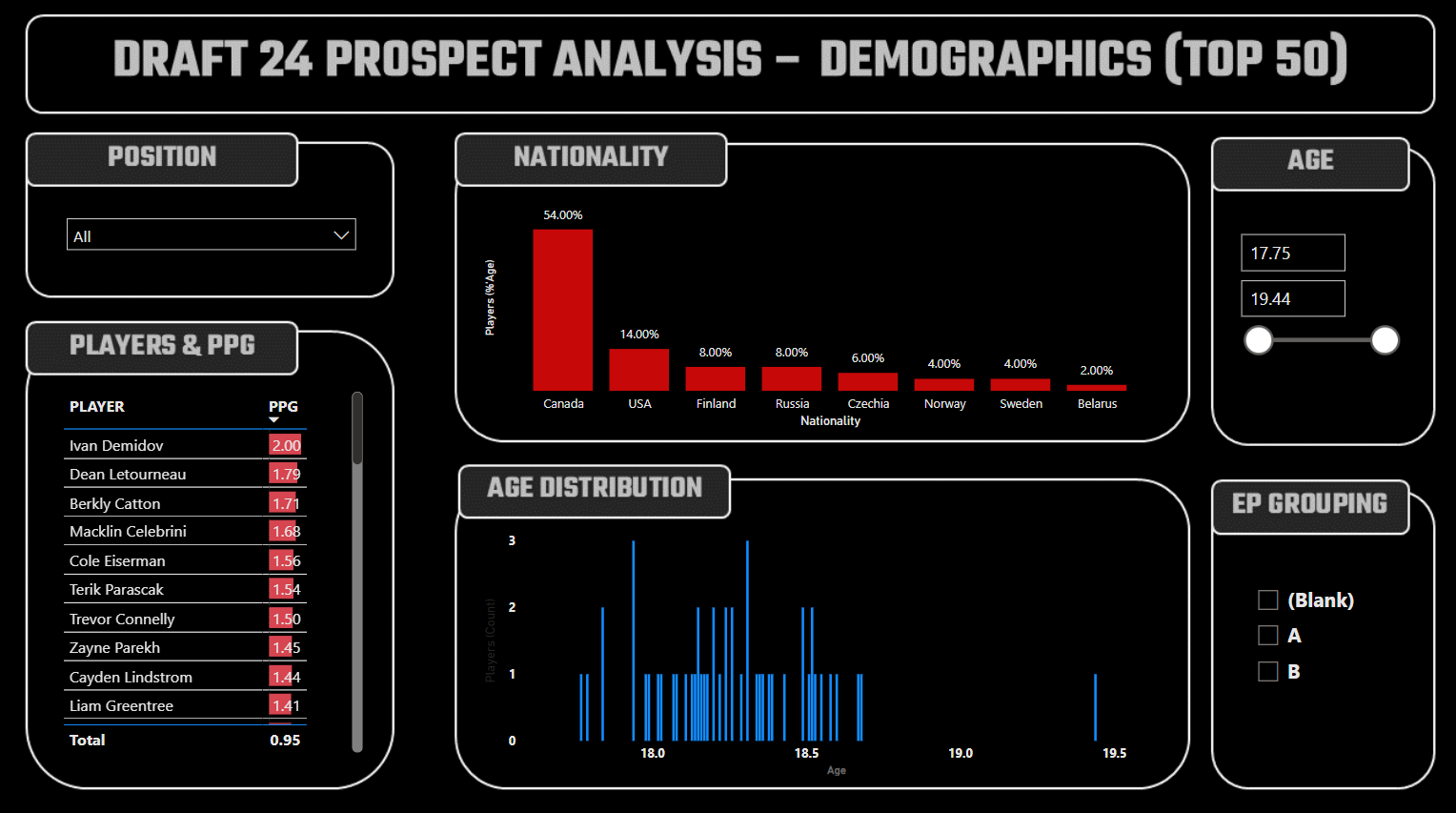
The next report we created was the Demographics report. Note that in this week's report, we included the Elite Prospects Grouping (EP_GROUPING). Given we only took the top 50, you'll only see Groups A and part of Group B.

The Demographics Report includes six controls:

1. Three Slicers, one for POSITION, one for AGE and one for EP_GROUPING.
2. One Table with two columns: PLAYER and PPG.
3. One Clustered Column Chart with NATIONALITY as the X-axis and PLAYER as the Y-axis. (The Y-axis is configured to be Percentage of Total.)
4. One Area Chart with AGE as the X-axis and PLAYER as the Y-axis – leaving the default as Count for PLAYER.

The below is what the final report looks like. This report is interactive, so you can use the Slicer controls to constrain the viewable data and then click parts of the main charts/tables to focus in one area or specific players.

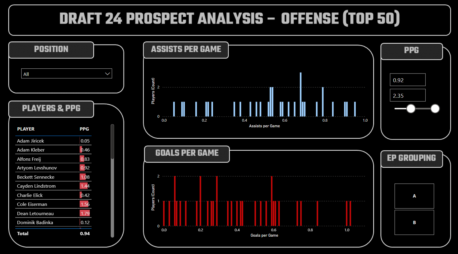
The Offense Report likewise includes six controls:

1. Three Slicers, one for POSITION, one for PPG and one for EP_GROUPING.
2. One Table with two columns: PLAYER and PPG.
3. One Clustered Column Chart with APG as the X-axis and PLAYER as the Y-axis.
4. A second Clustered Column Chart with GPG as the X-axis and PLAYER as the Y-axis.

The layout and design are similar to the other reports, and here again you can constrain the data to be viewed and then click on different parts of the charts and table to really focus on specific players or statistics.

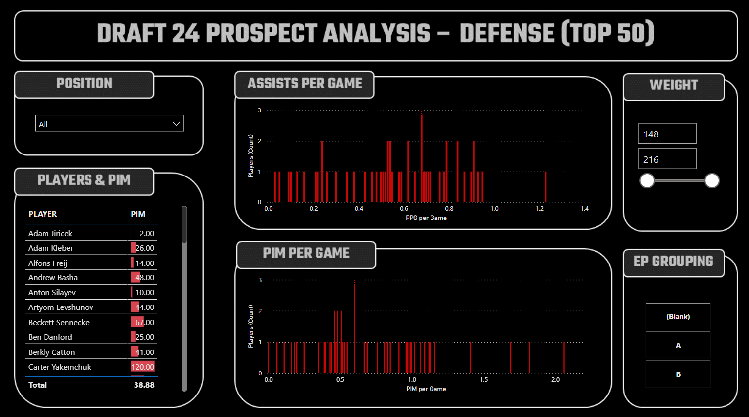
The Defense Report includes six controls:

1. Three Slicers including one for POSITION, one for WEIGHT and one for EP_GROUPING.
2. One Table with two columns: PLAYER and PIM.
3. One Clustered Column Chart with PPG as the X-axis and PLAYER as the Y-axis.
4. A second Clustered Column Chart with PIMPG as the X-axis and PLAYER as the Y-axis.

The design for this chart was a bit different from Week 4 because we felt it would be appropriate to include weight as an additional filter.

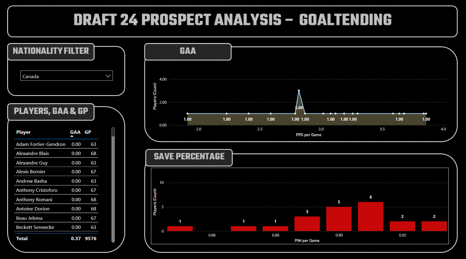
Because the top 50 prospects only include skaters, we have a Goaltending report, but it uses the broader prospect data but is filtered for G (POSITION).

The Goaltending Report includes four controls:

1. One Slicer for NATIONALITY.
2. One Table with three columns: PLAYER, GAA and GP.
3. One Area Chart with GAA as the X-axis and PLAYER as the Y-axis.
4. One Clustered Column Chart with SAVE_PCT as the X-axis and PLAYER as the Y-axis.

The below is the report for Goaltending.

You can download and explore the dashboard from here.

You can also check out our quick-hit YouTube video below:

Summary

In this week's newsletter edition (Week 5 in our six-week Preparing for the NHL Draft 2024 series), we analyzed the top 50 prospects (from the Elite Prospect's NHL 2024 Draft Guide). We split this analysis into two parts. The first part was an Exploratory Data Analysis, and the second was an interactive Power BI dashboard.

The downloads for this week are below:

• Top 50 Prospects Dataset
• Top 50 Power BI Dashboard

We recommend using the Top 50 Prospects dataset to explore the data with the data discovery techniques we've covered (e.g., sorting, filtering, etc.). Also, extend the Top 50 Power BI dashboard with your own design, reports, etc. You should ideally have the following at the end of your own work:

• Multiple datasets you can use for your own analyses
• Exploratory analyses in Microsoft Excel
• Prospect reports in Microsoft Power BI

Also, be sure to use the above to explore and compare the incoming prospects and use the Elite Prospects Draft 2024 Guide to get deeper assessments, scouting commentary and rating from the excellent work the Elite Prospects team has done to create this guide.

In Week 6, we will close the series by mapping the top prospects to the team analysis we did earlier in the newsletter series. We'll also create a presentation as an exercise to show how we would represent our findings/recommendations.

Subscribe to our newsletter to get the latest and greatest content on all things hockey analytics!