Build Your First Winning DFS Report using Microsoft Excel

In this Edition

• DFS Fantasy Hockey Series Recap
• Summary of Winning DFS Report
• Curating the Data
• Creating the Winning DFS Strategy Report

DFS Fantasy Hockey Series Recap

This is Week four in our six-week newsletter series on Winning in DFS Fantasy Hockey using Analytics. To date, we've covered the following topics:

• Week 1: DFS Fantasy Hockey 101: Your Ultimate Kickoff Guide!
• Week 2: Winning DFS Strategies & Stats to Crush Fantasy Hockey
• Week 3: More Winning Strategies & Statistics for DFS Hockey

In this week's edition, we'll take the first step in creating a report to demonstrate how we can take a strategy, map statistics to it in a data view and transform that view into a report that improves the odds of making winning decisions for your fantasy hockey lineup. We'll model the report after the High Shot Volume Player strategy.

Summary of Winning DFS Report

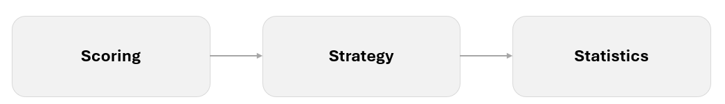
To create the report, we'll implement our DFS System that we introduced in an earlier newsletter – basically mapping scoring to strategy to statistics.

The report we'll build this week is modeled as follows:

• Scoring: We'll build a report that maps against the following DraftKings scoring:
  • Goals: +8.5 points
  • Assists: +5 points
  • Shots on Goal: +1.5 points
  • Blocked Shots: +1.3 points
• Strategy: We will build the report against the High Shot Volume Player strategy.
• Statistics: We'll use these statistics for the report:
  • Goals
  • Assists
  • Games Played
  • Shots on Goal
  • Shot Attempts
  • Shot Percentage
  • Blocked Shots

The goal of creating this report is to demonstrate how to curate, clean and transform data (that is freely available for you to use) and build a report that aids in your decision making each time you're evaluating your DFS lineup. There are of course more strategies to cover, so think of this report as your first step towards building out your own analytics-driven DFS system.

Let's get started!

Curating the Data

To implement this report, we're going to find and curate three seasons worth of data. A single, current season is okay to get the most recent statistics; however, you'll also want to build historical trending to see how a player performs over time. Further, having more data opens up your options to analyze the data in different ways – e.g., top-ranked players across seasons, variability patterns across seasons, and so on.

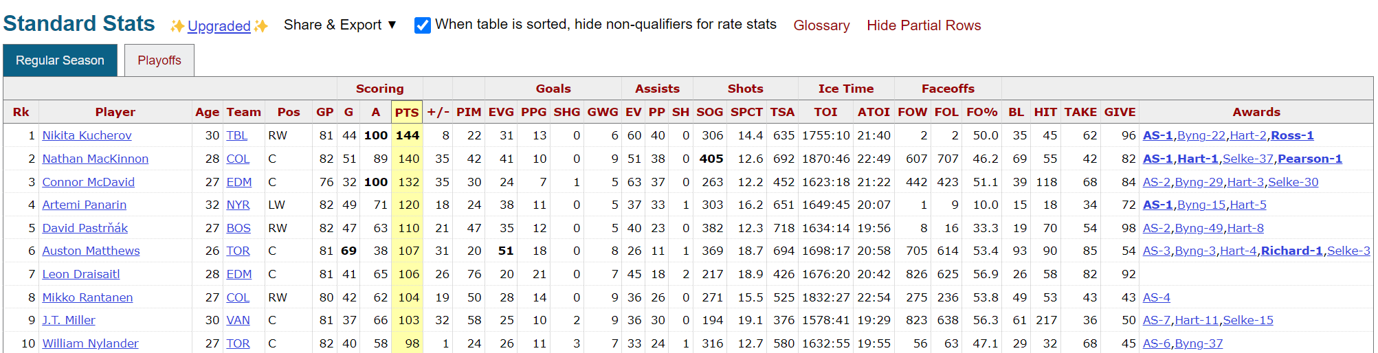
For this report, we'll use freely available data: skater statistics from Hockey-Reference. We use Hockey-Reference a lot because they have a ton of great hockey data, including some statistics that you won't readily find elsewhere. They also have data across multiple seasons, which you can export/download the data in easy-to-consume formats. For example, if you navigate to the 2023-2024 NHL Skater Statistics page, you'll find a Standard Stats table halfway down the page. You can explore the data on the page and mouse over the column headers to get more information on the statistics.

For this newsletter, we used their data from the Regular Season from 2021-2022, 2022-2023, and 2023-2024. The pages for these standard statistics are below:

• 2021-2022 NHL Skater Statistics
• 2022-2023 NHL Skater Statistics
• 2023-2024 NHL Skater Statistics

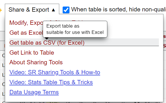
For each of the tables, we clicked Share & Export and then clicked Get table as CSV (for Excel). We then created three separate CSV files, which we compiled into one multi-season CSV file (we'll walk through how we did this in the next section).

Lastly, we curated a dataset that only included the top quartile of top shooters in the NHL – irrespective of position. Our reasoning: higher shots (especially on goal) have a positive correlation to goals. You may choose to get all players so you can look for "value players" who may have decent statistics but whose salary cap is lower.

Creating the Winning DFS Strategy Report

Three steps comprise the report-creation process:

1. Cleaning and transforming the data we downloaded from the Hockey-Ref website.
2. Creating a view in Microsoft Excel with the key stats.
3. Adding the DFS points into the Excel report.

The end result will be a simple Excel report that you can use to explore which players could land the most DFS points within your lineup.

We've posted several files that you can use for your own experimentation:

• All Player Data (from Hockey-Reference)
• Top Quartile of Players by SOG (from Hockey-Reference)
• R Code for Data Cleaning and Transformation
• High Shot Volume Player DFS Report

Cleaning & Transforming the Data

You can use Excel's data connectors and PowerQuery to link directly to the table in Hockey-Reference if you want. However, we prefer more programmatic control over the data. So, we did our own data cleaning and transformation in R and RStudio. Below are the core code snippets with short explanations of each snippet.

This first code snippet loads the libraries that you'll use for this application.

library(dbplyr)
library(tidyverse)

Next, we load the three CSV files we downloaded from Hockey-Reference into three different data frames.

player_summary_stats_2021_2022 <- read.csv("Hockey_Ref_Stats_Data_2021_2022.csv") 
player_summary_stats_2022_2023 <- read.csv("Hockey_Ref_Stats_Data_2022_2023.csv") 
player_summary_stats_2023_2024 <- read.csv("Hockey_Ref_Stats_Data_2023_2024.csv") 

This next code snippet implements some column heading transformation by using a function, into which we pass each data frame. We then add one column for each of the seasons to make sure we can identify data from a specific season later on down the line.

rename_columns <- function(df, new_names) {
  if(length(new_names) != ncol(df)) {
    stop("The length of new_names must match the number of columns in the data frame.")
  }
  
  colnames(df) <- new_names
  
  return(df)
}

new_names <- c("RANK", "PLAYER", "AGE", "TEAM", "POS", "GP", "G", "A", "PTS", "PLUS_MIN", 
               "PIM", "EVG", "PPG", "SHG", "GWG", "EV", "PP", "SH", "SOG", "SHOT_PCT",
               "TSA", "TOI", "ATOI", "FOW", "FOL", "FO_PCT", "BL", "HITS", "TAKE", "GIVE", "AWARDS")

player_summary_stats_2021_2022_df <- rename_columns(player_summary_stats_2021_2022, new_names)
player_summary_stats_2022_2023_df <- rename_columns(player_summary_stats_2022_2023, new_names)
player_summary_stats_2023_2024_df <- rename_columns(player_summary_stats_2023_2024, new_names)

player_summary_stats_2021_2022_df$SEASON = "2021_2022"
player_summary_stats_2022_2023_df$SEASON = "2022_2023"
player_summary_stats_2023_2024_df$SEASON = "2023_2024"

This next code snippet combines the data frames into a single data frame using the rbind() function.

all_player_summary_stats_data_df <- rbind(player_summary_stats_2021_2022_df, player_summary_stats_2022_2023_df, player_summary_stats_2023_2024_df)

We then trim the dataset to the statistics that we need.

player_data_for_analysis <- all_player_summary_stats_data_df %>% 
  select(SEASON, PLAYER, AGE, TEAM, POS, GP, G, A, PTS, PIM, EVG, PPG, SHG, GWG, EV, PP, SH, SOG, SHOT_PCT, TSA, TOI, ATOI, FOW, FOL, FO_PCT, BL, HITS, TAKE, GIVE)
  

The next code snippet creates a new data frame (using the trimmed data frame) that breaks the players into quartiles. This is based off of Shots on Goal (SOG).

quartile_view <- player_data_for_analysis %>%
  group_by(SEASON) %>%
  summarise(
    Q1 = quantile(SOG, 0.25, na.rm = TRUE),   
    Median = quantile(SOG, 0.50, na.rm = TRUE),   
    Q3 = quantile(SOG, 0.75, na.rm = TRUE), 
    Q4 = quantile(SOG, 1.0, na.rm = TRUE),
  )

And finally, we create a data frame with only those players that are in the top quartile.

quartile_thresholds <- player_data_for_analysis %>%
  group_by(SEASON) %>%
  summarise(Q3 = quantile(SOG, 0.75, na.rm = TRUE))

df_with_q3 <- player_data_for_analysis %>%
  left_join(quartile_thresholds, by = "SEASON")

players_in_q3 <- df_with_q3 %>%
  filter(SOG >= Q3)

The resulting CSV is a dataset with three seasons worth of player data that contain only the top shooters (i.e., all shooters from the top quartile). This is what we will now use to create the report in Microsoft Excel.

Creating a View in Microsoft Excel

The workbook in Excel is composed of two tabs: All_Data and DFS_Report. The All_Data tab will have all of the top quartile data that we filtered on in the R code (shown in the last section). The DFS_Report tab will focus on a narrower set of hockey statistics that map to our High Shot Volume Player strategy. That is:

• Goals (G)
• Assists (A)
• Games Played (GP)
• Shots on Goal (SOG)
• Shot Attempts (TSA)
• Shot Percentage (SHOT_PCT)
• Blocked Shots (BL)

Let's first work through a couple of steps to create the data view with the above data, and then we'll complete the report in the next section by adding the point calculations against DraftKings point system.

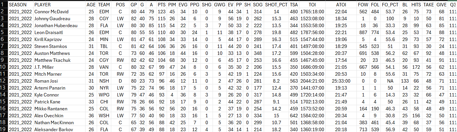
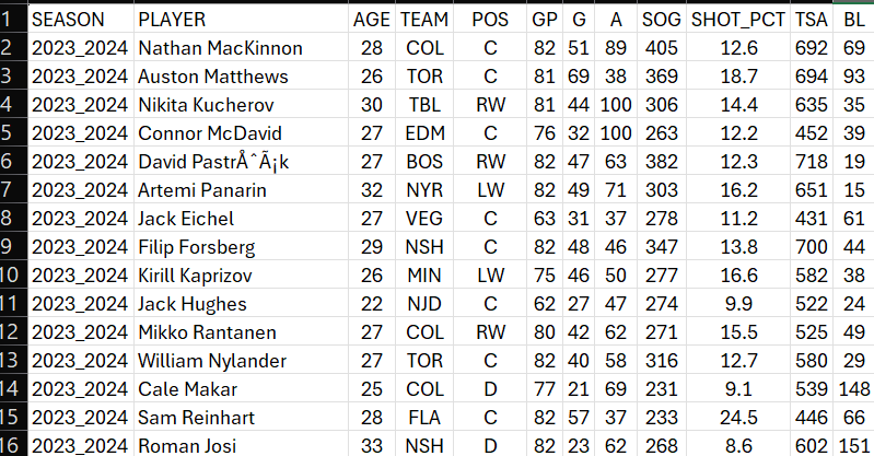
The first step is open the Top Quartile of Shooters CSV file and save it as an Excel Workbook with a new name. When you open the CSV in Excel (or your preferred spreadsheet program), you'll see the following rows and columns.

As a general part of our process, we keep one tab with all of the data in it and then copy and paste the data we need into another tab. So, create a new tab in the Excel workbook called DFS_Report and copy over the columns you see below.

Next, click the cell in the upper top-left corner of the worksheet and click the Home tab on the ribbon, Format as Table, select a style and the cell range and click OK. You now have the starting point for your DFS Report.

Adding the DFS Points Calculation

With the DFS_Report tab now hydrated with filtered hockey statistics, you'll now do four things:

1. Calculate the "per game" stats.
2. Calculate the DFS points against the per game stats (using DraftKings scoring model).
3. Add conditional formatting to create a heatmap report for your statistics of choice.
4. Add a slicer to help you focus on specific teams and positions when you're evaluating for your lineup.

We're targeting four point statistics from DraftKings scoring model: Goals, Assists, Shots on Goal, and Blocked Shots. So, we'll be creating eight new columns, four for the per game statistic and four for the DFS point calculation – so steps 1 and 2 above.

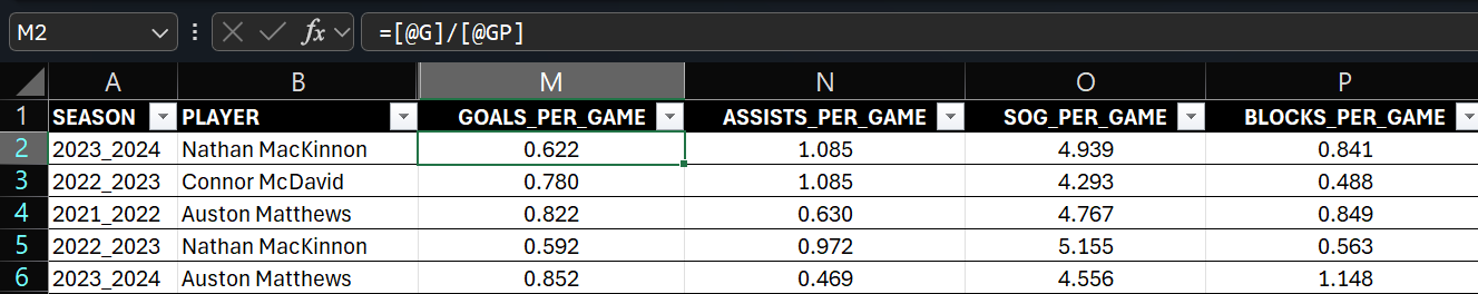
To add the per game stats, click the cell beside BL (the column heading cell) and type GOALS_PER_GAME. When you're done, Excel automatically adds this column to the formatted table. You'll now add a formula to calculate the goals per game, which is Goals divided by Games Played or =[@G]/[@GP]. When you create this for the top cell in the column, Excel will autofill the rest of the cells in that column. Repeat the above step for ASSISTS_PER_GAME, SOG_PER_GAME and BLOCKED_PER_GAME. After you do this, you'll have four additional columns that have an average hockey statistic calculated based on the number of games that a player has played.

When done, you should have something similar to the below.

Next, you'll repeat the same process as above (i.e., click the cell to the right of the last one and add a formula into the cell) for the cells that will calculate the DFS points for you. You can call these cells: DFS_GOALS, DFS_ASSISTS, DFS_SOG, and DFS_BLOCKED. These cells will calculate the average points (based on DraftKings scoring model) using the per game statistics you just created. So, the formulae for each of the cells are as follows:

• DFS_GOALS: =[@[GOALS_PER_GAME]]*8.5
• DFS_ASSISTS: =[@[ASSISTS_PER_GAME]]*5
• DFS_SOG: =[@[SOG_PER_GAME]]*1.5
• DFS_BLOCKED: =[@[BLOCKED_PER_GAME]]*1.3

You should now have all the columns you need for the key scores for each player.

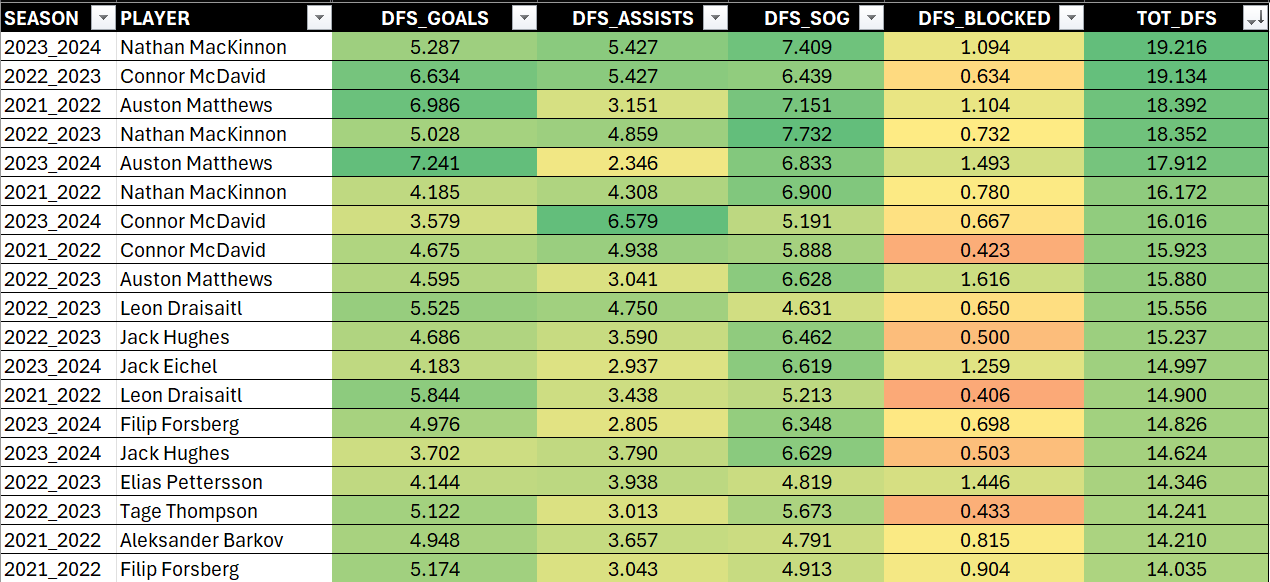
You are now ready to add the conditional formatting to your data view. You can select those columns that you want to use for your heatmap; we created the heatmap using the per game statistics and the DFS points columns. To do this, click the Home tab on the ribbon, select the cells you want to conditionally format, and select Conditional Formatting, Color Scales and select the specific color scale you want.

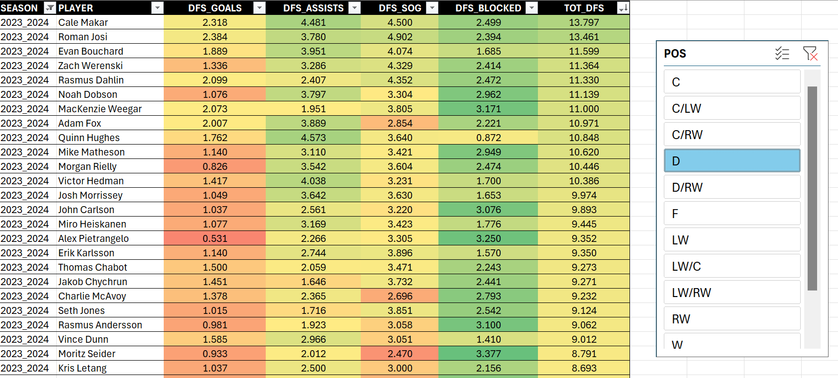
When done, you'll see something similar to the below. And while it may appear a bit unwieldly to look at, the key is to understand green is better than red within the heatmap. So, when you explore the DFS point columns, you can sort from largest to smallest and you should then see the players who would have better potential to get you higher DFS points.

The final step is to add a slicer to filter the view down, so you can quickly navigate the report to get to target teams or positions. To do this, click the Insert tab on the ribbon and then click Slicer. You can then select the columns you want to use to create your slicer, e.g., TEAM and POS for teams and position, respectively.

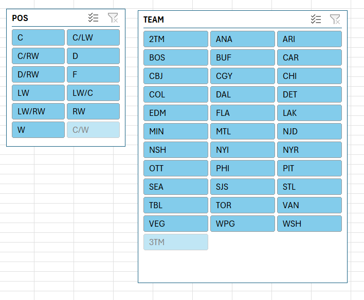
You can now use this report when making decisions about your DFS lineup. For example, you want to find the top defenseman to include in your picks from this season, you filter SEASON on 2023_2024 and D using the slicer and then sort on the appropriate columns to find the player that can maximize your DFS point gain.

And there you go! Your very first DFS Report that maps to the High Shot Volume Player strategy – and even gives you more point gains based on other metrics as well.

If you just want to download the finished report, then you can get it here. We'd recommend spending some time exploring and experimenting with the report, so you can extend it, map it to your own strategies, and so on.

Check out our quick-hit YouTube video that walks through the above at the following link:

Summary

This was the fourth newsletter in our six-part series on building an analytically-driven winning DFS system for fantasy hockey. In this newsletter, we walked you through how to create an Excel-based DFS report that was modeled against the High Shot Volume Player strategy and used four scores within the DraftKings scoring system (Goals, Assists, Shots on Goal and Blocked Shots).

The pros of this report are that it's based on freely available data, and you can quickly curate the data and create a report that is easy to use in Excel. You can also create a report that gives you a simple way to calculate the DFS point gain for specific players based on their past performance.

The cons of this report are that it's based on summary data (more granular, game-based data would be more ideal), and we didn't build any cross- or intra-season trending into the report. So, there are limitations within the report that we'd want to think through. Some of this can be done using PivotTables (which you can explore using the data and report files) and some of this can be done using different tools, such as Power BI – which would give you a more fully-featured experience.

In our next newsletter, we'll expand our analytically-driven DFS system to include other strategies and implement the system in Power BI. This will give us the chance to explore and represent more strategies and statistics through the features that Power BI has to offer.

Subscribe to our newsletter to get the latest and greatest content on all things hockey analytics!